Stomatal Conductance and Plant Transpiration

This article is a primer on water vapor transpiration in plants, one of the most important phenomena in the hydrologic cycle. We begin with a brief discussion concerning stomata, the adjustable pores that mediate gas exchange between leaves and the atmosphere. A quick overview of the stomatal opening mechanism and the factors that affect it is provided. The resistance/conductance of stomata and other components of the gas-exchange pathway are presented, and the text closes with a simple set of calculations involving these parameters.

1. Stomatal anatomy and aperture

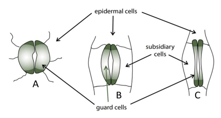
Stomatal anatomy varies from one plant to the next, and more primitive species often have less refined stomata. Figure 1, extracted from Willey’s Environmental Plant Physiology, illustrates the stomata of three types of plants. Illustration A shows the stomata of primitive plants, which have no dedicated subsidiary cells and produce a relatively small cavity even when guard cells are turgid. Illustration B shows the stomata of many angiosperms, in which case the guard cells are accompanied by subsidiary cells that work together to produce a larger cavity. Illustration C shows the stomata of the grass Triticum aestivum, whose dumbbell-shaped guard cells operate in tandem with the subsidiary cells to open along their length, maximizing the area of the stoma. Grasses have characteristic guard cells and rapidly responding accessory cells, factors that partially explain their high water use efficiency (WUE).

Figure 1. Anatomy of stomata.

At full opening, the stomatal apertures of Phaseolus vulgaris (bean plant) measure 3 $\displaystyle \times$ 7 $\displaystyle \mu$ m, while fully open stomata of Zebrina pendula (inchplant) reach pore sizes of 12 $\displaystyle \times$ 31 $\displaystyle \mu$ m. In the Poaceae (grass) family, stomata are particularly elongate – a fully open stomatal pore of Avena sativa (oat) measures 8 $\displaystyle \times$ 38 $\displaystyle \mu$ m. The number of stomata (mm^-2 leaf area) varies widely between species, and may be as low as 30 (Triticum, Laryx) to over 5000 (Impatiens). Usually no more than 3% of leaf surface area is covered with stomatal cavities.

The stomatal aperture is controlled by the conformation of the two guard cells surrounding a pore. These cells are generally kidney-shaped, may be 40 $\displaystyle \mu$ m long, and, unlike ordinary epidermal cells, usually contain chloroplasts. When the guard cells are relatively flaccid, the stomatal pore is nearly closed, as is the case of most plants at night. Upon illumination, guard cells take up K⁺, which may increase in concentration from 0.2 M to 0.5 M. The uptake of potassium raises the internal osmotic pressure, thus lowering the internal water potential; water then spontaneously flows from the epidermal cells into the guard cells by osmosis. This water entry leads to an increase in the internal hydrostatic pressure of a pair of guard cells, causing them to expand and their cell walls on either side of the pore to become concave. As the kidney-shaped guard cells bow outward, an elliptical pore develops between the two cells. The formation of this pore is a consequence of the anisotropy of the cell wall surrounding each guard cell, as the elastic properties vary with direction. The distance between the guard cells across the open pore (the pore “width”) is usually 5 to 15 $\displaystyle \mu$ m, and the major axis along the elliptical pore can be about 20 $\displaystyle \mu$ m. The water relations of the special epidermal cells immediately surrounding the guard cells, the subsidiary cells, are also crucial for stomatal opening. For instance, K⁺ and Cl^– can move from the subsidiary cells to the guard cells, causing water to leave the subsidiary cells and their internal hydrostatic pressure to decrease while that of guard cells increases. The foregoing effects on stomatal aperture are summarized in Figure 2.

Figure 2. Opening and closure of stomata. Effects in blue chronologically occur from top to bottom.

It was long assumed that stomata respond homogeneously over the entire leaf. However, leaves of water-stressed plants exposed to ¹⁴CO₂ often show a heterogeneous distribution of fixed ¹⁴C. This shows that some stomata close completely (there is no radioactivity close to these stomata), whereas others hardly change their aperture (radioactive label is located near these stomata). This patchiness of stomatal closure can also be visualized dynamically and nondestructively with thermal and chlorophyll fluorescence imaging techniques.

2. Factors that affect stomatal opening

Several factors affect stomatal opening or closure to varying degrees. Some are briefly discussed below.

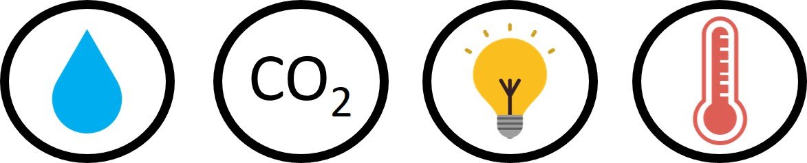
Atmospheric humidity: In addition to assimilating carbon dioxide, stomata also mediate transpiration of water vapor to the atmosphere. The water vapor content within the leaf is usually close to saturation. So, a dry atmosphere gives rise to a large gradient in water vapor across the stomatal pore, that is, a leaf-to-air vapor pressure deficit (VPD), which increases as the relative humidity outside falls. Increasing VPD leads to a proportional increase in transpiration rate through the stomatal pore, driven by diffusion. Stomata therefore generally close at high VPD to prevent excessive water loss.

Carbon dioxide: Stomata react to the gradient of CO₂ concentration between the external air and the intercellular spaces of leaves. Decreasing CO₂ concentration in ambient air causes stomata to open, while increasing it causes stomata to close. The degree of stomatal opening often depends on the concentration of CO₂ in the guard cells, which reflects their own carbohydrate metabolism as well as the CO₂ level in the air within the leaf. For instance, upon illumination the CO₂ concentration in the leaf intercellular air spaces is decreased by photosynthesis, resulting in decreased CO₂ levels in the guard cells, which triggers stomatal opening. CO₂ can then enter the leaf and photosynthesis can continue.

Light: The photoreceptors in stomatal cells can perceive certain light wavelengths, especially in the blue region of the visible spectrum. Activated by such receptors, stomata open with increasing light intensity. Stomatal conductance in the morning increases earlier than photosynthesis, which is only activated when the sun has risen further and with a larger proportion of red light. Therefore, stomatal opening caused by light does not adversely limit the flow of CO₂ for photosynthesis during the day.

Temperature: Stomata close at low temperatures and open at higher temperatures. Increasing temperature can override the closing effects of increased CO₂ levels and darkness. For example, increasing the temperature from 27^oC to 36^oC resulted in stomatal opening of Xanthum leaves in the dark without removal of CO₂.

3. Stomatal resistance/conductance

We now turn to the resistance/conductance that each component of the leaf-atmosphere pathway offers to water vapor flow. Reference values are given in Table 1. The stomata are an obvious first choice for discussion. In the simplest case of a circular cylinder or other shape of circular cross-section, the resistance of the stomatal pore is given by $\displaystyle {{r}^{{st}}}$ = $\displaystyle \ell$ /D, where $\displaystyle \ell$ is the length of the cylinder and D is the diffusion coefficient. This resistance per unit pore area can be converted to a resistance per unit area of leaf by dividing by the ratio of average pore cross-sectional area to leaf surface area. For circular pores this ratio is $\displaystyle v\pi {{r}^{2}}$ , where $\displaystyle v$ is the frequency of stomata per unit leaf area and $\displaystyle r$ is the pore radius. The stomatal resistance on a leaf area basis then becomes

$\displaystyle {{r}^{{st}}}=\frac{\ell }{{v\pi {{r}^{2}}D}}$

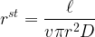
Because the pore area is much less than the leaf area, there is a zone close to the pore where the lines of flux converge on the pore. Therefore, this zone of the boundary layer is not effectively utilized and there is an extra resistance or ‘end effect’ associated with each pore. The magnitude of this extra resistance can be derived from three-dimensional diffusion theory to be proportional to the pore radius and ultimately equal to $\displaystyle \pi r$ /4D. Accordingly, converting to a leaf area basis and accounting for the extra pore resistance, we write

$\displaystyle {{r}^{{st}}}=\frac{{\ell +{{\pi r}}/{4}\;}}{{v\pi {{r}^{2}}D}}$

As an example, suppose we wish to determine the stomatal diffusion resistance and the corresponding conductance for water vapor flow on a leaf with 225 stomata/mm² on each surface, each pore being 12 $\displaystyle \text{ }\!\!\mu\!\!\text{ }$ m deep and circular in cross-section with diameter of 5 $\displaystyle \text{ }\!\!\mu\!\!\text{ }$ m. The ambient temperature is 20ºC, at which the corresponding diffusion coefficient for water vapor in air is 24.2 $\displaystyle \times$ 10^-6m²/s (see, e.g., The Engineering Toolbox). All we have to do is substitute the pertinent data in the previous equation, giving

$\displaystyle {{r}^{{st}}}=\frac{{12\times {{{10}}^{{-6}}}+\pi \times {{\left( {2.5\times {{{10}}^{{-6}}}} \right)}}/{4}\;}}{{\left( {225\times {{{10}}^{6}}} \right)\times \pi \times {{{\left( {2.5\times {{{10}}^{{-6}}}} \right)}}^{2}}\times \left( {24.2\times {{{10}}^{{-6}}}} \right)}}=131\,\text{s}\,{{\text{m}}^{{-1}}}\leftarrow$

For each surface, $\displaystyle {{{r}'}^{{st}}}$ = 131/2 = 65.5 s m^-1. The conductance $\displaystyle {{{g}'}^{{st}}}$ is then

$\displaystyle {{{g}'}^{{st}}}=\frac{1}{{{{{{r}'}}^{{st}}}}}=\frac{1}{{65.5}}=1.53\times {{10}^{{-2}}}\,\text{m}\,{{\text{s}}^{{-1}}}=15.3\,\text{mm}\,\,{{\text{s}}^{{-1}}}\leftarrow$

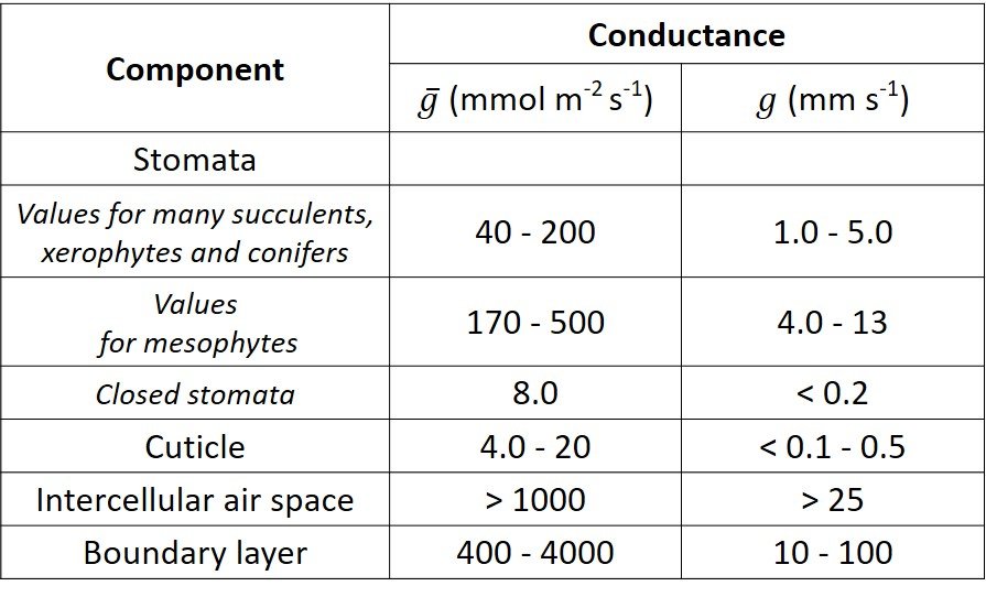
Table 1. Typical conductance values for components of the leaf-atmosphere pathway

4. Other conductances/resistances

Some water molecules diffuse across the waxy cuticle of the epidermal cells; we can thus speak of cuticular transpiration, which involves both liquid water and water vapor. The cuticle is in parallel with the stomata, which is to say that water vapor can leave the leaf either by crossing the cuticle or by going through the stomatal pores. The conductance for cuticular transpiration, $\displaystyle g_{{wv}}^{c}$ , usually ranges from 0.1 to 0.5 mm/s. Cuticular conductance is often much smaller than $\displaystyle g_{{wv}}^{{st}}$ for open stomata, but can exceed it when stomata are nearly closed. Although the cuticular resistance tends to be by far the highest component of leaf resistance, the resistance tends to be dominated by the stomatal component because the resistance of two parallel resistors is determined primarily by the smaller one.

Another conductance to consider in the diffusion of water vapor in plant leaves is that of the intercellular air spaces, which usually account for about 30% of the leaf volume. Its value can be calculated with the ratio

$\displaystyle g_{{wv}}^{{ias}}=\frac{D}{{{{\delta }^{{ias}}}}}$

where D is the diffusion coefficient of water vapor in air and $\displaystyle {{\delta }^{{ias}}}$ is a representative equivalent length that usually varies from 100 $\displaystyle \text{ }\!\!\mu\!\!\text{ }$ m to 1 mm, yielding a conductance between 25 and 250 mm/s at average temperatures.

The fourth and last conductance/resistance component we must account for stems from the boundary layer, the thin stratum of disturbed airflow located between the surface of the leaf and the free-stream air. The thickness of the boundary layer is affected by the roughness of the leaf, the wind speed, and the distance along the leaf. Its contribution to resistance is relatively small. For a deeper insight on boundary layers in external flow, refer to one of our free materials on transport phenomena.

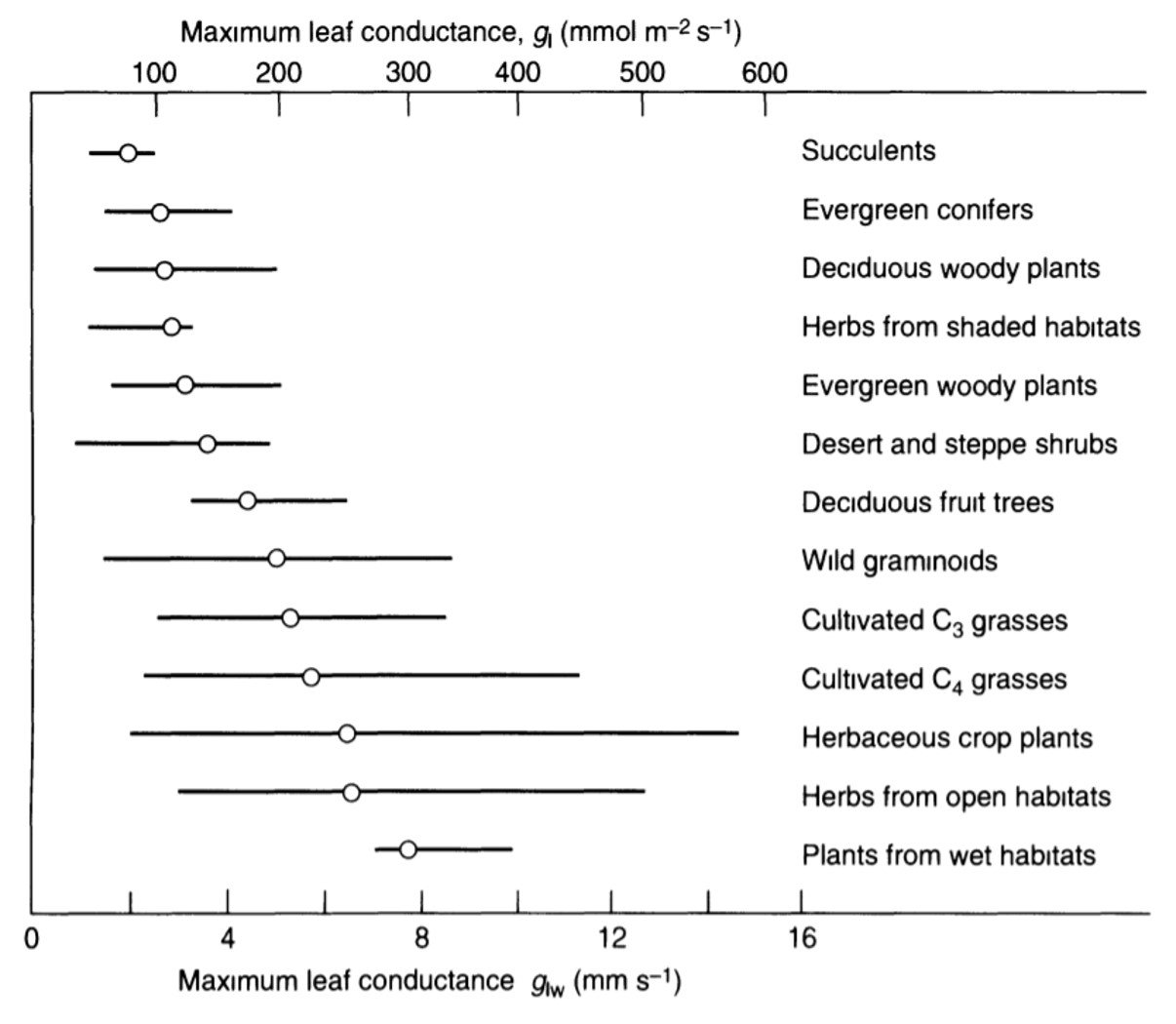
Three of the foregoing conductance components – stomatal, cuticular, and intercellular air space – together constitute the leaf conductance. Some values for leaves of select species are given in Figure 3.

Figure 3. Maximum leaf conductance in different groups of plants. The lines cover about 90% of individual values reported, and the open circles represent group average conductances.

We have thus introduced the four conductance/resistance components involved in flow of water vapor across a leaf. As noted by Nobel (2009), two such components are strictly anatomical (intercellular air spaces and cuticle), one depends on anatomy and yet responds to metabolical as well as environmental factors (stomata), and one depends on leaf morphology and wind speed (boundary layer). We can assemble a hypothetical conductance pathway to represent flow of water vapor across the leaf, as shown in Figure 4.

Figure 4. Conductance arrangement for water vapor transpiration.

Let $\displaystyle \text{g}_{{wv}}^{{ias}}$ denote the intercellular air spaces conductance, $\displaystyle \text{g}_{{wv}}^{{st}}$ the stomatal conductance, $\displaystyle \text{g}_{{wv}}^{c}$ the cuticular conductance, and $\displaystyle \text{g}_{{wv}}^{{bl}}$ the boundary layer conductance. Because the water vapor conductance of the intercellular air spaces and the stomata are in series, their equivalent conductance is $\displaystyle \text{g}_{{wv}}^{{ias}}g_{{wv}}^{{st}}$ /( $\displaystyle \text{g}_{{wv}}^{{ias}}$ + $\displaystyle g_{{wv}}^{{st}}$ ). These two conductances are associated in parallel to the cuticular conductance, so that the vapor conductance of the leaf is expressed as

$\displaystyle g_{{wv}}^{{leaf}}=\frac{{g_{{wv}}^{{ias}}g_{{wv}}^{{st}}}}{{g_{{wv}}^{{ias}}+g_{{wv}}^{{st}}}}+g_{{wv}}^{c}$

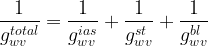
Next, we note that the leaf conductance $\displaystyle g_{{wv}}^{{leaf}}$ is in series with the boundary layer conductance $\displaystyle g_{{wv}}^{{bl}}$ , and that the two sides of a leaf act as parallel conductances for water vapor diffusing from the interior of a leaf. We therefore obtain the following expression for the total conductance of a leaf with air boundary layers on each side,

$\displaystyle g_{{wv}}^{{total}}=\frac{{g_{{wv}}^{{lea{{f}_{u}}}}g_{{wv}}^{{b{{l}_{u}}}}}}{{g_{{wv}}^{{lea{{f}_{u}}}}+g_{{wv}}^{{b{{l}_{u}}}}}}+\frac{{g_{{wv}}^{{lea{{f}_{l}}}}g_{{wv}}^{{b{{l}_{l}}}}}}{{g_{{wv}}^{{lea{{f}_{l}}}}+g_{{wv}}^{{b{{l}_{l}}}}}}$

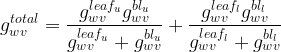
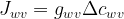
Having obtained the conductances, we can establish the net flux density $\displaystyle {{J}_{i}}$ of water vapor between any two regions of interest. We generally express gas fluxes on the basis of unit area of one side of a leaf. Assuming one-dimensional Fickian diffusion to be valid, the water vapor net flux density $\displaystyle {{J}_{{wv}}}$ can be estimated as

$\displaystyle {{J}_{{wv}}}={{g}_{{wv}}}\Delta {{c}_{{wv}}}$

where $\displaystyle \Delta {{c}_{{wv}}}$ is the water vapor concentration gradient between two points of interest. The variation in saturation values of water vapor concentration is given in Figure 5. We can also express the relation above with the difference in mole fractions, $\displaystyle \Delta {{N}_{{wv}}}$ , as the driving force for diffusion. Denoting $\displaystyle {{\bar{g}}_{{wv}}}$ as the molar-basis conductance, we write

$\displaystyle {{\bar{J}}_{{wv}}}={{\bar{g}}_{{wv}}}\Delta {{N}_{{wv}}}$

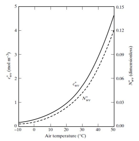
The mole fraction of water vapor can also be read from Figure 5.

Figure 5. Variation in saturation values of water vapor concentration ( $\displaystyle c_{{wv}}^{*}$ ) and mole fraction ( $\displaystyle N_{{wv}}^{*}$ ) with temperature. Ambient air pressure was assumed to be 1 atm.

Example (Modified from Nobel, 2009)

Suppose a leaf has the following conductances.

• Conductance of water vapor in the lower-surface boundary layer, $\displaystyle g_{{wv}}^{{b{{l}_{l}}}}$ = 24 mm/s;

• Conductance of water vapor in the lower-surface stomata, $\displaystyle g_{{wv}}^{{s{{t}_{l}}}}$ = 7.5 mm/s;

• Conductance of water vapor in cuticle, $\displaystyle g_{{wv}}^{c}$ = 0.2 mm/s;

• Conductance of water vapor in intercellular air spaces, $\displaystyle g_{{wv}}^{{ias}}$ = 40 mm/s;

A) What is $\displaystyle g_{{wv}}^{{total}}$ if water vapor diffuses out only across the lower epidermis of the leaf?

B) What would be the $\displaystyle g_{{wv}}^{{total}}$ values in A if (i) the cuticular pathway is ignored; (ii) the intercellular air spaces are ignored; or (iii) both the cuticular and intercellular space pathways are ignored?

C) What is $\displaystyle g_{{wv}}^{{total}}$ if the stomata in the upper epidermis have the same conductance as those in the lower epidermis?

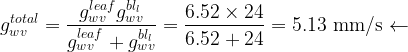
D) What is the total water vapor conductance if 30% of the diffusion flux is through the upper epidermis?

E) Suppose that the leaf temperature is 30^oC, the air in the cell wall pores where the water evaporates is at 90% relative humidity, and the turbulent air water vapor concentration $\displaystyle c_{{wv}}^{{ta}}$ is 7 g/m³. What is the diffusion flux through the lower epidermis?

F) What are $\displaystyle \bar{g}_{{wv}}^{{total}}$ in mmol m^-2 s^-1 and $\displaystyle {{\bar{J}}_{{wv}}}$ in mmol m^-2 s^-1 under the conditions posited in part E? Assume that the air pressure is 1 atm and that the molar fraction of water vapor in turbulent air, $\displaystyle N_{{wv}}^{{ta}}$ , is 0.0105.

A) We begin by calculating the water vapor conductance of the leaf,

$\displaystyle g_{{wv}}^{{leaf}}=\frac{{g_{{wv}}^{{ias}}g_{{wv}}^{{st}}}}{{g_{{wv}}^{{ias}}+g_{{wv}}^{{st}}}}+g_{{wv}}^{c}$

$\displaystyle \therefore g_{{wv}}^{{leaf}}=\frac{{40\times 7.5}}{{40+7.5}}+0.2=6.52\,\,\text{mm/s}$

The total conductance of the leaf, observing that water vapor diffuses out only across the lower surface of the leaf, is then

$\displaystyle g_{{wv}}^{{total}}=\frac{{g_{{wv}}^{{leaf}}g_{{wv}}^{{b{{l}_{l}}}}}}{{g_{{wv}}^{{leaf}}+g_{{wv}}^{{b{{l}_{l}}}}}}=\frac{{6.52\times 24}}{{6.52+24}}=5.13\,\,\text{mm/s}\leftarrow$

B) If the cuticular pathway is ignored, the remaining three conductances are connected in series; that is,

$\displaystyle \frac{1}{{g_{{wv}}^{{total}}}}=\frac{1}{{g_{{wv}}^{{ias}}}}+\frac{1}{{g_{{wv}}^{{st}}}}+\frac{1}{{g_{{wv}}^{{bl}}}}$

$\displaystyle \therefore \frac{1}{{g_{{wv}}^{{total}}}}=\frac{1}{{40}}+\frac{1}{{7.5}}+\frac{1}{{24}}$

$\displaystyle \therefore g_{{wv}}^{{total}}=5\,\,\text{mm/s}\leftarrow$

If the intercellular air spaces are ignored, stomatal and cuticular conductances are in parallel ( $\displaystyle g_{{wv}}^{{leaf}}$ = $\displaystyle g_{{wv}}^{{st}}$ + $\displaystyle g_{{wv}}^{c}$ ) and in series with the boundary layer conductance. Thus,

$\displaystyle g_{{wv}}^{{leaf}}=7.5+0.2=7.7\,\,\text{mm/s}$

and

$\displaystyle \frac{1}{{g_{{wv}}^{{total}}}}=\frac{1}{{g_{{wv}}^{{leaf}}}}+\frac{1}{{g_{{wv}}^{{bl}}}}$

$\displaystyle \therefore \frac{1}{{g_{{wv}}^{{total}}}}=\frac{1}{{7.7}}+\frac{1}{{24}}$

$\displaystyle \therefore g_{{wv}}^{{total}}=5.83\,\,\text{mm/s}\leftarrow$

If both cuticular and intercellular air spaces are ignored, we are left with a series connection of stomatal and boundary layer conductances, so that

$\displaystyle \frac{1}{{g_{{wv}}^{{total}}}}=\frac{1}{{g_{{wv}}^{{st}}}}+\frac{1}{{g_{{wv}}^{{bl}}}}$

$\displaystyle \therefore \frac{1}{{g_{{wv}}^{{total}}}}=\frac{1}{{7.5}}+\frac{1}{{24}}$

$\displaystyle \therefore g_{{wv}}^{{total}}=5.71\,\,\text{mm/s}\leftarrow$

C) The conductance of the upper surface here equals the conductance of the lower surface, determined in A, and is in parallel with it. In mathematical terms,

$\displaystyle g_{{wv}}^{{total}}=g_{{wv}}^{u}+g_{{wv}}^{l}=5.13+5.13=10.3\,\,\text{mm/s}\leftarrow$

D) In this case, 70% of the diffusion flux stems from the lower epidermis. Using the total conductance calculated in part A, it follows that

$\displaystyle g_{{wv}}^{{total}}=\frac{{g_{{wv}}^{l}}}{{0.7}}=\frac{{5.13}}{{0.7}}=7.33\,\,\text{mm/s}\leftarrow$

E) The diffusion flux is given by

$\displaystyle J_{{wv}}^{l}=g_{{wv}}^{{total}}\Delta c_{{wv}}^{{total}}=g_{{wv}}^{{total}}\left( {c_{{wv}}^{{leaf}}-c_{{wv}}^{{ta}}} \right)$

Conductance $\displaystyle g_{{wv}}^{{total}}$ = 5.13 mm/s was determined in part A. The turbulent air water vapor concentration $\displaystyle c_{{wv}}^{{ta}}$ = 7 g/m³. Concentration $\displaystyle c_{{wv}}^{{leaf}}$ depends on the relative humidity RH = 90% and the saturated water vapor concentration for a temperature of 30^oC, which can be read from Figure 5 to be about 1.7 mol/m³ or, equivalently, 30.6 g/m³. Thus, $\displaystyle c_{{wv}}^{{leaf}}$ = 0.90 $\displaystyle \times$ 30.6 = 27.5 g/m³, so that

$\displaystyle J_{{wv}}^{l}=g_{{wv}}^{{total}}\Delta c_{{wv}}^{{total}}=g_{{wv}}^{{total}}\left( {c_{{wv}}^{{leaf}}-c_{{wv}}^{{ta}}} \right)=5.13\times \left( {27.5-7} \right)=105\,\,\text{mg}\,{{\text{m}}^{{-2}}}\,{{\text{s}}^{{-1}}}\leftarrow$

F) Appealing to the ideal gas law and noting that 1 m³ = 1000 L, we have

$\displaystyle \bar{g}_{{wv}}^{{total}}=g_{{wv}}^{{total}}\frac{P}{{RT}}=\left( {5.13\times {{{10}}^{{-3}}}} \right)\times \frac{{1.0}}{{0.0821\times 303}}\times 1000=0.206\,\ \text{mol}\,{{\text{m}}^{{-2}}}{{\text{s}}^{{-1}}}$

$\displaystyle \therefore \bar{g}_{{wv}}^{{total}}=206\,\ \text{mmol}\,{{\text{m}}^{{-2}}}{{\text{s}}^{{-1}}}$

Referring to the dotted curve in Figure 5, we read a mole fraction $\displaystyle N_{{wv}}^{{leaf}}$ = 0.04. It remains to compute the molar flux density,

$\displaystyle {{\bar{J}}_{{wv}}}=\bar{g}_{{wv}}^{{total}}\left( {N_{{wv}}^{{total}}-N_{{wv}}^{{ta}}} \right)$
$\displaystyle \therefore {{\bar{J}}_{{wv}}}=206\times \left( {0.04-0.0105} \right)=6.08\,\text{mmol }{{\text{m}}^{{-2}}}\,{{\text{s}}^{{-1}}}\leftarrow$

References

• JONES, H. (2014). Plants and Microclimate. 3rd edition. Cambridge: Cambridge University Press.

• LAMBERS, H., CHAPIN III, F., and PONS, T. (2008). Plant Physiological Ecology. 2nd edition. Berlin/Heidelberg: Springer.

• NOBEL, P. (2009). Physicochemical and Environmental Plant Physiology. 4th edition. London: Academic Press.

• WILLEY, N. (2016). Environmental Plant Physiology. New York: Garland Science.

• WILLMER, C. and FRICKER, M. (1996). Stomata. 2nd edition. Berlin/Heidelberg: Springer.

Stomatal Conductance and Plant Transpiration

Subscribe to our Mailing List!

Featured Posts

A Primer on NAND Flash Memories

Solidification Time and Chvorinov’s Rule

Step-Growth Polymerization, the Carothers Equation, and the Flory-Schulz Distribution

More Articles

The Bruun Rule and Sea-Level Rise

Glacier Profiles: The Parabolic, Vialov, and Bueler Models

Fields of Study

More

© 2024 Montogue Quiz

Subscribe to
our Mailing List!

Subscribe to our Mailing List!

Subscribe to receive our latest materials in your inbox.

Homework Help

© 2024 Montogue Quiz

Subscribe to our Mailing List!