In this article, we investigate single-reaction gas-phase equilibria; specifically, we show how one can easily determine the equilibrium composition with knowledge of the equilibrium constant K. As the student surely knows, any typical chemical reaction can be represented by the general notation

where 


the stoichiometric numbers are

The number of moles 

where we have introduced a variable 
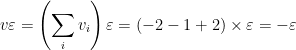
Summation over all species yields
The mole fractions 

In a gas-phase reaction, the molar fractions, the system presure, and the so-called equilibrium constant are related by an expression of the form
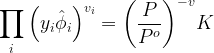
Here, 


In words, the scary product on the left-hand side simply means that we should multiply in series the molar fractions of each component i, taken to a power equal to its stoichiometric coefficient. Consider, for instance, the simple equilibrium

Here, 


The molar fractions can be shown to be

so that

Clearly, determining the extent of reaction

The value of 

Here, subscript “0” denotes a quantity expressed at the reference temperature 


![\displaystyle \int_{{{{T}_{0}}}}^{T}{{\frac{{\Delta C_{p}^{\text{o}}}}{R}\frac{{dT}}{T}}}=\Delta A\ln \tau +\left[ {\Delta B{{T}_{0}}+\left( {\Delta CT_{0}^{2}+\frac{{\Delta D}}{{{{\tau }^{2}}T_{0}^{2}}}} \right)\left( {\frac{{\tau +1}}{2}} \right)} \right]\left( {\tau -1} \right)](https://s0.wp.com/latex.php?latex=%5Cdisplaystyle+%5Cint_%7B%7B%7B%7BT%7D_%7B0%7D%7D%7D%7D%5E%7BT%7D%7B%7B%5Cfrac%7B%7B%5CDelta+C_%7Bp%7D%5E%7B%5Ctext%7Bo%7D%7D%7D%7D%7BR%7D%5Cfrac%7B%7BdT%7D%7D%7BT%7D%7D%7D%3D%5CDelta+A%5Cln+%5Ctau+%2B%5Cleft%5B+%7B%5CDelta+B%7B%7BT%7D_%7B0%7D%7D%2B%5Cleft%28+%7B%5CDelta+CT_%7B0%7D%5E%7B2%7D%2B%5Cfrac%7B%7B%5CDelta+D%7D%7D%7B%7B%7B%7B%5Ctau+%7D%5E%7B2%7D%7DT_%7B0%7D%5E%7B2%7D%7D%7D%7D+%5Cright%29%5Cleft%28+%7B%5Cfrac%7B%7B%5Ctau+%2B1%7D%7D%7B2%7D%7D+%5Cright%29%7D+%5Cright%5D%5Cleft%28+%7B%5Ctau+-1%7D+%5Cright%29&bg=ffffff&fg=000&s=0&c=20201002)
in which 


Having evaluated all terms on the right-hand side of equation (III), the reaction change in Gibbs free energy 
Step 1. With the initial number of moles and stoichiometric coefficients, determine expressions for the molar fractions using equation (I).
Step 2. Substitute the molar fractions into equation (II) to determine an expression that relates the extent of reaction
Step 3. Determine the heat of reaction
Step 4. Using the temperature ratio
Step 5. Using the results from steps 3 and 4, determine the right-hand side of equation (III).
Step 6. Knowing that 
Step 7. Substituting K in the expression determined in step 2, determine the extent of reaction
Step 8. Substitute
We now present two applied examples.
Example 1
The following reaction reaches equilibrium at 500ºC and 2 bar:

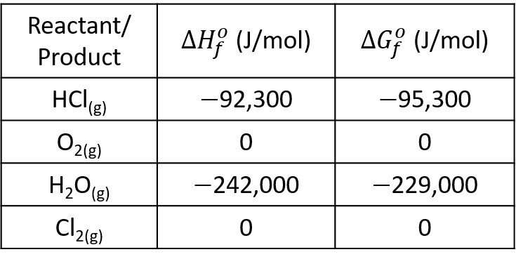
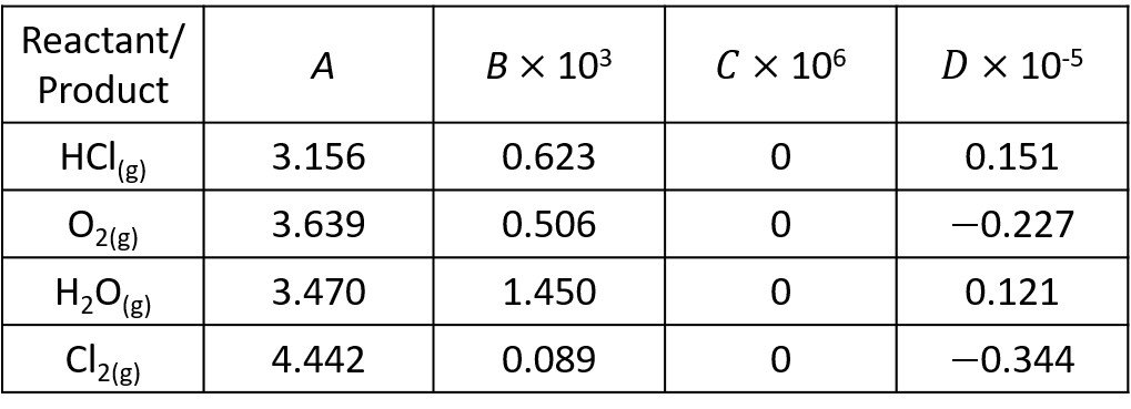
If the system initially contains 5 mol of HCl for each mole of oxygen, what is the composition of the system at equilibrium? Assume ideal gases. Use the following data.
The molar balance is outlined below.
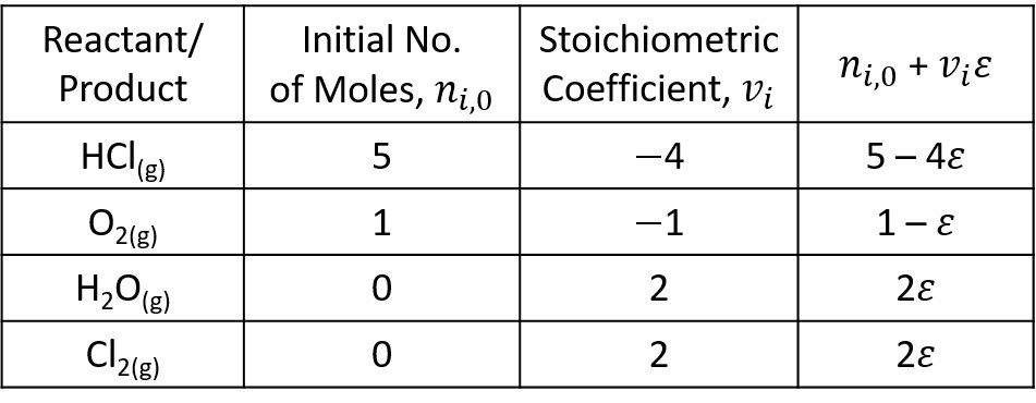
The total No. of moles at the beginning of the reaction is

The product of reaction stoichiometric number and extent of reaction is

The mole fractions of each component are written next.


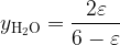

The equilibrium constant, pressure, and composition are related by equation (II),
Substituting the molar fractions,

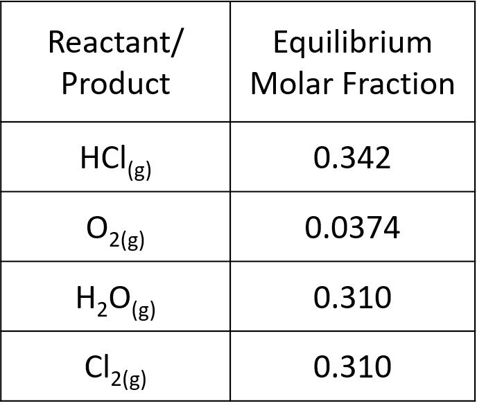
It remains to compute the equilibrium constant K. In step 3, we calculate the heat of reaction at 298 K,
![\displaystyle \Delta H_{{298}}^{\text{o}}=\left[ {2\Delta H_{{f,298}}^{\text{o}}\left( {{{\text{H}}_{\text{2}}}\text{O}} \right)+2\Delta H_{{f,298}}^{\text{o}}\left( {\text{C}{{\text{l}}_{\text{2}}}} \right)} \right]-\left[ {4\Delta H_{{f,298}}^{\text{o}}\left( {\text{HCl}} \right)+\Delta H_{{f,298}}^{\text{o}}\left( {{{\text{O}}_{\text{2}}}} \right)} \right]](https://s0.wp.com/latex.php?latex=%5Cdisplaystyle+%5CDelta+H_%7B%7B298%7D%7D%5E%7B%5Ctext%7Bo%7D%7D%3D%5Cleft%5B+%7B2%5CDelta+H_%7B%7Bf%2C298%7D%7D%5E%7B%5Ctext%7Bo%7D%7D%5Cleft%28+%7B%7B%7B%5Ctext%7BH%7D%7D_%7B%5Ctext%7B2%7D%7D%7D%5Ctext%7BO%7D%7D+%5Cright%29%2B2%5CDelta+H_%7B%7Bf%2C298%7D%7D%5E%7B%5Ctext%7Bo%7D%7D%5Cleft%28+%7B%5Ctext%7BC%7D%7B%7B%5Ctext%7Bl%7D%7D_%7B%5Ctext%7B2%7D%7D%7D%7D+%5Cright%29%7D+%5Cright%5D-%5Cleft%5B+%7B4%5CDelta+H_%7B%7Bf%2C298%7D%7D%5E%7B%5Ctext%7Bo%7D%7D%5Cleft%28+%7B%5Ctext%7BHCl%7D%7D+%5Cright%29%2B%5CDelta+H_%7B%7Bf%2C298%7D%7D%5E%7B%5Ctext%7Bo%7D%7D%5Cleft%28+%7B%7B%7B%5Ctext%7BO%7D%7D_%7B%5Ctext%7B2%7D%7D%7D%7D+%5Cright%29%7D+%5Cright%5D&bg=ffffff&fg=000&s=0&c=20201002)
![\displaystyle \therefore \Delta H_{{298}}^{\text{o}}=\left[ {2\times \left( {-242,000} \right)+2\times 0} \right]-\left[ {4\times \left( {-92,300} \right)+0} \right]=-114,800\,\,\text{J/mol}](https://s0.wp.com/latex.php?latex=%5Cdisplaystyle+%5Ctherefore+%5CDelta+H_%7B%7B298%7D%7D%5E%7B%5Ctext%7Bo%7D%7D%3D%5Cleft%5B+%7B2%5Ctimes+%5Cleft%28+%7B-242%2C000%7D+%5Cright%29%2B2%5Ctimes+0%7D+%5Cright%5D-%5Cleft%5B+%7B4%5Ctimes+%5Cleft%28+%7B-92%2C300%7D+%5Cright%29%2B0%7D+%5Cright%5D%3D-114%2C800%5C%2C%5C%2C%5Ctext%7BJ%2Fmol%7D&bg=ffffff&fg=000&s=0&c=20201002)
and the change in Gibbs free energy at 298 K,
![\displaystyle \Delta G_{{298}}^{\text{o}}=\left[ {2\Delta G_{{f,298}}^{\text{o}}\left( {{{\text{H}}_{\text{2}}}\text{O}} \right)+2\Delta G_{{f,298}}^{\text{o}}\left( {\text{C}{{\text{l}}_{\text{2}}}} \right)} \right]-\left[ {4\Delta G_{{f,298}}^{\text{o}}\left( {\text{HCl}} \right)+\Delta G_{{f,298}}^{\text{o}}\left( {{{\text{O}}_{\text{2}}}} \right)} \right]](https://s0.wp.com/latex.php?latex=%5Cdisplaystyle+%5CDelta+G_%7B%7B298%7D%7D%5E%7B%5Ctext%7Bo%7D%7D%3D%5Cleft%5B+%7B2%5CDelta+G_%7B%7Bf%2C298%7D%7D%5E%7B%5Ctext%7Bo%7D%7D%5Cleft%28+%7B%7B%7B%5Ctext%7BH%7D%7D_%7B%5Ctext%7B2%7D%7D%7D%5Ctext%7BO%7D%7D+%5Cright%29%2B2%5CDelta+G_%7B%7Bf%2C298%7D%7D%5E%7B%5Ctext%7Bo%7D%7D%5Cleft%28+%7B%5Ctext%7BC%7D%7B%7B%5Ctext%7Bl%7D%7D_%7B%5Ctext%7B2%7D%7D%7D%7D+%5Cright%29%7D+%5Cright%5D-%5Cleft%5B+%7B4%5CDelta+G_%7B%7Bf%2C298%7D%7D%5E%7B%5Ctext%7Bo%7D%7D%5Cleft%28+%7B%5Ctext%7BHCl%7D%7D+%5Cright%29%2B%5CDelta+G_%7B%7Bf%2C298%7D%7D%5E%7B%5Ctext%7Bo%7D%7D%5Cleft%28+%7B%7B%7B%5Ctext%7BO%7D%7D_%7B%5Ctext%7B2%7D%7D%7D%7D+%5Cright%29%7D+%5Cright%5D&bg=ffffff&fg=000&s=0&c=20201002)
![\displaystyle \therefore \Delta G_{{298}}^{\text{o}}=\left[ {2\times \left( {-229,000} \right)+2\times 0} \right]-\left[ {4\times \left( {-95,300} \right)+0} \right]=-76,800\,\,\text{J/mol}](https://s0.wp.com/latex.php?latex=%5Cdisplaystyle+%5Ctherefore+%5CDelta+G_%7B%7B298%7D%7D%5E%7B%5Ctext%7Bo%7D%7D%3D%5Cleft%5B+%7B2%5Ctimes+%5Cleft%28+%7B-229%2C000%7D+%5Cright%29%2B2%5Ctimes+0%7D+%5Cright%5D-%5Cleft%5B+%7B4%5Ctimes+%5Cleft%28+%7B-95%2C300%7D+%5Cright%29%2B0%7D+%5Cright%5D%3D-76%2C800%5C%2C%5C%2C%5Ctext%7BJ%2Fmol%7D&bg=ffffff&fg=000&s=0&c=20201002)
Next, we compute the 


![\displaystyle \,\Delta D=\sum\limits_{i}^{\,}{{{{v}_{i}}{{D}_{i}}}}=\left[ {2\times 0.121+2\times \left( {-0.344} \right)-4\times 0.151-1\times \left( {-0.227} \right)} \right]\times {{10}^{5}}=-8.23\times {{10}^{4}}](https://s0.wp.com/latex.php?latex=%5Cdisplaystyle+%5C%2C%5CDelta+D%3D%5Csum%5Climits_%7Bi%7D%5E%7B%5C%2C%7D%7B%7B%7B%7Bv%7D_%7Bi%7D%7D%7B%7BD%7D_%7Bi%7D%7D%7D%7D%3D%5Cleft%5B+%7B2%5Ctimes+0.121%2B2%5Ctimes+%5Cleft%28+%7B-0.344%7D+%5Cright%29-4%5Ctimes+0.151-1%5Ctimes+%5Cleft%28+%7B-0.227%7D+%5Cright%29%7D+%5Cright%5D%5Ctimes+%7B%7B10%7D%5E%7B5%7D%7D%3D-8.23%5Ctimes+%7B%7B10%7D%5E%7B4%7D%7D&bg=ffffff&fg=000&s=0&c=20201002)
Now, the temperature ratio is


and the entropy integral
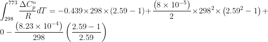
![\displaystyle \int_{{298}}^{{773}}{{\frac{{\Delta {{C}_{p}}}}{R}\frac{{dT}}{T}}}=\Delta A\ln \tau +\left[ {\Delta B{{T}_{0}}+\left( {\Delta CT_{0}^{2}+\frac{{\Delta D}}{{{{\tau }^{2}}T_{0}^{2}}}} \right)\left( {\frac{{\tau +1}}{2}} \right)} \right]\left( {\tau -1} \right)](https://s0.wp.com/latex.php?latex=%5Cdisplaystyle+%5Cint_%7B%7B298%7D%7D%5E%7B%7B773%7D%7D%7B%7B%5Cfrac%7B%7B%5CDelta+%7B%7BC%7D_%7Bp%7D%7D%7D%7D%7BR%7D%5Cfrac%7B%7BdT%7D%7D%7BT%7D%7D%7D%3D%5CDelta+A%5Cln+%5Ctau+%2B%5Cleft%5B+%7B%5CDelta+B%7B%7BT%7D_%7B0%7D%7D%2B%5Cleft%28+%7B%5CDelta+CT_%7B0%7D%5E%7B2%7D%2B%5Cfrac%7B%7B%5CDelta+D%7D%7D%7B%7B%7B%7B%5Ctau+%7D%5E%7B2%7D%7DT_%7B0%7D%5E%7B2%7D%7D%7D%7D+%5Cright%29%5Cleft%28+%7B%5Cfrac%7B%7B%5Ctau+%2B1%7D%7D%7B2%7D%7D+%5Cright%29%7D+%5Cright%5D%5Cleft%28+%7B%5Ctau+-1%7D+%5Cright%29&bg=ffffff&fg=000&s=0&c=20201002)
![\displaystyle \therefore \int_{{298}}^{{773}}{{\frac{{\Delta C_{p}^{\text{o}}}}{R}\frac{{dT}}{T}}}=-0.439\times \ln \left( {2.59} \right)+\left[ {\left( {8\times {{{10}}^{{-5}}}} \right)\times 298+\left( {0-\frac{{8.23\times {{{10}}^{4}}}}{{{{{2.59}}^{2}}\times {{{298}}^{2}}}}} \right)\left( {\frac{{2.59+1}}{2}} \right)} \right]\left( {2.59-1} \right)](https://s0.wp.com/latex.php?latex=%5Cdisplaystyle+%5Ctherefore+%5Cint_%7B%7B298%7D%7D%5E%7B%7B773%7D%7D%7B%7B%5Cfrac%7B%7B%5CDelta+C_%7Bp%7D%5E%7B%5Ctext%7Bo%7D%7D%7D%7D%7BR%7D%5Cfrac%7B%7BdT%7D%7D%7BT%7D%7D%7D%3D-0.439%5Ctimes+%5Cln+%5Cleft%28+%7B2.59%7D+%5Cright%29%2B%5Cleft%5B+%7B%5Cleft%28+%7B8%5Ctimes+%7B%7B%7B10%7D%7D%5E%7B%7B-5%7D%7D%7D%7D+%5Cright%29%5Ctimes+298%2B%5Cleft%28+%7B0-%5Cfrac%7B%7B8.23%5Ctimes+%7B%7B%7B10%7D%7D%5E%7B4%7D%7D%7D%7D%7B%7B%7B%7B%7B2.59%7D%7D%5E%7B2%7D%7D%5Ctimes+%7B%7B%7B298%7D%7D%5E%7B2%7D%7D%7D%7D%7D+%5Cright%29%5Cleft%28+%7B%5Cfrac%7B%7B2.59%2B1%7D%7D%7B2%7D%7D+%5Cright%29%7D+%5Cright%5D%5Cleft%28+%7B2.59-1%7D+%5Cright%29&bg=ffffff&fg=000&s=0&c=20201002)

We now have all the information necessary to calculate 


Resolving the logarithm,

Substituting in equation (IV) yields

Adjusting the fraction on the left-hand side, we have

The equation above is a fifth-degree polynomial in
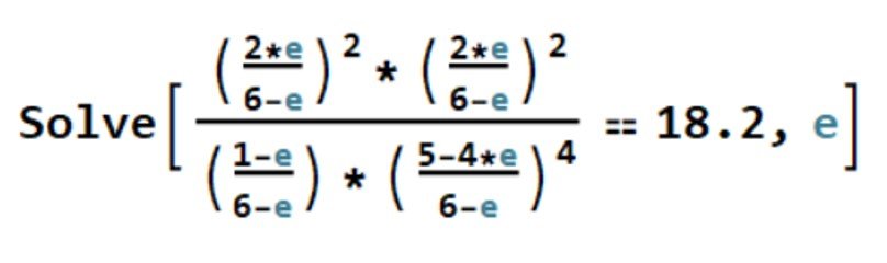
This returns four imaginary solutions and


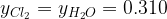
The sum of molar fractions is such that

as it should be. The slight difference is due to roundoff. Our results are tabulated below.
Example 2
Oil refineries frequently have both 


For reactants in the stoichiometric proportion, estimate the molar fraction of each reactant if the reaction comes to equilibrium at 450ºC and 8 bar. Use the following data.
The sulfur exists pure as a solid phase, for which the activity is 

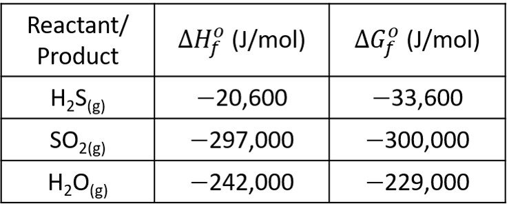
The total No. of moles at the beginning of the reaction is

The product of reaction stoichiometric number and extent of reaction is
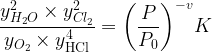
The mole fractions of each component are written next.
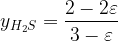
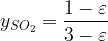

The equilibrium constant, pressure, and composition are related by equation (II),
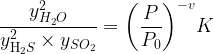
Substituting the molar fractions,
The heat of reaction at 298 K is
![\displaystyle \Delta H_{{298}}^{\text{o}}=\left[ {2\Delta H_{{f,298}}^{\text{o}}\left( {{{\text{H}}_{\text{2}}}\text{O}} \right)} \right]-\left[ {2\Delta H_{{f,298}}^{\text{o}}\left( {{{\text{H}}_{\text{2}}}\text{S}} \right)+\Delta H_{{f,298}}^{\text{o}}\left( {\text{S}{{\text{O}}_{\text{2}}}} \right)} \right]](https://s0.wp.com/latex.php?latex=%5Cdisplaystyle+%5CDelta+H_%7B%7B298%7D%7D%5E%7B%5Ctext%7Bo%7D%7D%3D%5Cleft%5B+%7B2%5CDelta+H_%7B%7Bf%2C298%7D%7D%5E%7B%5Ctext%7Bo%7D%7D%5Cleft%28+%7B%7B%7B%5Ctext%7BH%7D%7D_%7B%5Ctext%7B2%7D%7D%7D%5Ctext%7BO%7D%7D+%5Cright%29%7D+%5Cright%5D-%5Cleft%5B+%7B2%5CDelta+H_%7B%7Bf%2C298%7D%7D%5E%7B%5Ctext%7Bo%7D%7D%5Cleft%28+%7B%7B%7B%5Ctext%7BH%7D%7D_%7B%5Ctext%7B2%7D%7D%7D%5Ctext%7BS%7D%7D+%5Cright%29%2B%5CDelta+H_%7B%7Bf%2C298%7D%7D%5E%7B%5Ctext%7Bo%7D%7D%5Cleft%28+%7B%5Ctext%7BS%7D%7B%7B%5Ctext%7BO%7D%7D_%7B%5Ctext%7B2%7D%7D%7D%7D+%5Cright%29%7D+%5Cright%5D&bg=ffffff&fg=000&s=0&c=20201002)
![\displaystyle \therefore \Delta H_{{298}}^{\text{o}}=\left[ {2\times \left( {-242,000} \right)} \right]-\left[ {2\times \left( {-20,600} \right)+\left( {-297,000} \right)} \right]=-145,800\,\,\text{J/mol}](https://s0.wp.com/latex.php?latex=%5Cdisplaystyle+%5Ctherefore+%5CDelta+H_%7B%7B298%7D%7D%5E%7B%5Ctext%7Bo%7D%7D%3D%5Cleft%5B+%7B2%5Ctimes+%5Cleft%28+%7B-242%2C000%7D+%5Cright%29%7D+%5Cright%5D-%5Cleft%5B+%7B2%5Ctimes+%5Cleft%28+%7B-20%2C600%7D+%5Cright%29%2B%5Cleft%28+%7B-297%2C000%7D+%5Cright%29%7D+%5Cright%5D%3D-145%2C800%5C%2C%5C%2C%5Ctext%7BJ%2Fmol%7D&bg=ffffff&fg=000&s=0&c=20201002)
and the change in Gibbs free energy at 298 K is
![\displaystyle \Delta G_{{298}}^{\text{o}}=\left[ {2\Delta G_{{f,298}}^{\text{o}}\left( {{{\text{H}}_{\text{2}}}\text{O}} \right)} \right]-\left[ {2\Delta G_{{f,298}}^{\text{o}}\left( {{{\text{H}}_{\text{2}}}\text{S}} \right)+\Delta G_{{f,298}}^{\text{o}}\left( {\text{S}{{\text{O}}_{\text{2}}}} \right)} \right]](https://s0.wp.com/latex.php?latex=%5Cdisplaystyle+%5CDelta+G_%7B%7B298%7D%7D%5E%7B%5Ctext%7Bo%7D%7D%3D%5Cleft%5B+%7B2%5CDelta+G_%7B%7Bf%2C298%7D%7D%5E%7B%5Ctext%7Bo%7D%7D%5Cleft%28+%7B%7B%7B%5Ctext%7BH%7D%7D_%7B%5Ctext%7B2%7D%7D%7D%5Ctext%7BO%7D%7D+%5Cright%29%7D+%5Cright%5D-%5Cleft%5B+%7B2%5CDelta+G_%7B%7Bf%2C298%7D%7D%5E%7B%5Ctext%7Bo%7D%7D%5Cleft%28+%7B%7B%7B%5Ctext%7BH%7D%7D_%7B%5Ctext%7B2%7D%7D%7D%5Ctext%7BS%7D%7D+%5Cright%29%2B%5CDelta+G_%7B%7Bf%2C298%7D%7D%5E%7B%5Ctext%7Bo%7D%7D%5Cleft%28+%7B%5Ctext%7BS%7D%7B%7B%5Ctext%7BO%7D%7D_%7B%5Ctext%7B2%7D%7D%7D%7D+%5Cright%29%7D+%5Cright%5D&bg=ffffff&fg=000&s=0&c=20201002)
![\displaystyle \therefore \Delta G_{{298}}^{\text{o}}=\left[ {2\times \left( {-229,000} \right)} \right]-\left[ {2\times \left( {-33,600} \right)+\left( {-300,000} \right)} \right]=-90,800\,\,\text{J/mol}](https://s0.wp.com/latex.php?latex=%5Cdisplaystyle+%5Ctherefore+%5CDelta+G_%7B%7B298%7D%7D%5E%7B%5Ctext%7Bo%7D%7D%3D%5Cleft%5B+%7B2%5Ctimes+%5Cleft%28+%7B-229%2C000%7D+%5Cright%29%7D+%5Cright%5D-%5Cleft%5B+%7B2%5Ctimes+%5Cleft%28+%7B-33%2C600%7D+%5Cright%29%2B%5Cleft%28+%7B-300%2C000%7D+%5Cright%29%7D+%5Cright%5D%3D-90%2C800%5C%2C%5C%2C%5Ctext%7BJ%2Fmol%7D&bg=ffffff&fg=000&s=0&c=20201002)
Next, we compute the

![\displaystyle \Delta B=\sum\limits_{i}{{{{v}_{i}}{{B}_{i}}}}=\left[ {2\times 1.490+3\times \left( {-1.728} \right)-2\times 1.450-1\times 0.801} \right]\times {{10}^{{-3}}}=-5.99\times {{10}^{{-3}}}](https://s0.wp.com/latex.php?latex=%5Cdisplaystyle+%5CDelta+B%3D%5Csum%5Climits_%7Bi%7D%7B%7B%7B%7Bv%7D_%7Bi%7D%7D%7B%7BB%7D_%7Bi%7D%7D%7D%7D%3D%5Cleft%5B+%7B2%5Ctimes+1.490%2B3%5Ctimes+%5Cleft%28+%7B-1.728%7D+%5Cright%29-2%5Ctimes+1.450-1%5Ctimes+0.801%7D+%5Cright%5D%5Ctimes+%7B%7B10%7D%5E%7B%7B-3%7D%7D%7D%3D-5.99%5Ctimes+%7B%7B10%7D%5E%7B%7B-3%7D%7D%7D&bg=ffffff&fg=000&s=0&c=20201002)

![\displaystyle \Delta D=\left[ {2\times 0.121+3\times \left( {-0.783} \right)-2\times \left( {-0.232} \right)-1\times \left( {-1.015} \right)} \right]\times {{10}^{5}}=-6.28\times {{10}^{4}}](https://s0.wp.com/latex.php?latex=%5Cdisplaystyle+%5CDelta+D%3D%5Cleft%5B+%7B2%5Ctimes+0.121%2B3%5Ctimes+%5Cleft%28+%7B-0.783%7D+%5Cright%29-2%5Ctimes+%5Cleft%28+%7B-0.232%7D+%5Cright%29-1%5Ctimes+%5Cleft%28+%7B-1.015%7D+%5Cright%29%7D+%5Cright%5D%5Ctimes+%7B%7B10%7D%5E%7B5%7D%7D%3D-6.28%5Ctimes+%7B%7B10%7D%5E%7B4%7D%7D&bg=ffffff&fg=000&s=0&c=20201002)
Now, the temperature ratio is
and the entropy integral
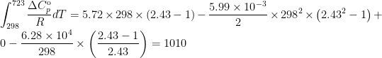
![\displaystyle \int_{{298}}^{{723}}{{\frac{{\Delta C_{p}^{\text{o}}}}{R}\frac{{dT}}{T}}}=5.72\times \ln \left( {2.43} \right)+\left[ {\left( {-5.99\times {{{10}}^{{-3}}}} \right)\times 298+\left( {0-\frac{{6.28\times {{{10}}^{4}}}}{{2.43\times {{{10}}^{2}}\times {{{298}}^{2}}}}} \right)\times \left( {\frac{{2.43+1}}{2}} \right)} \right]\times \left( {2.43-1} \right)](https://s0.wp.com/latex.php?latex=%5Cdisplaystyle+%5Cint_%7B%7B298%7D%7D%5E%7B%7B723%7D%7D%7B%7B%5Cfrac%7B%7B%5CDelta+C_%7Bp%7D%5E%7B%5Ctext%7Bo%7D%7D%7D%7D%7BR%7D%5Cfrac%7B%7BdT%7D%7D%7BT%7D%7D%7D%3D5.72%5Ctimes+%5Cln+%5Cleft%28+%7B2.43%7D+%5Cright%29%2B%5Cleft%5B+%7B%5Cleft%28+%7B-5.99%5Ctimes+%7B%7B%7B10%7D%7D%5E%7B%7B-3%7D%7D%7D%7D+%5Cright%29%5Ctimes+298%2B%5Cleft%28+%7B0-%5Cfrac%7B%7B6.28%5Ctimes+%7B%7B%7B10%7D%7D%5E%7B4%7D%7D%7D%7D%7B%7B2.43%5Ctimes+%7B%7B%7B10%7D%7D%5E%7B2%7D%7D%5Ctimes+%7B%7B%7B298%7D%7D%5E%7B2%7D%7D%7D%7D%7D+%5Cright%29%5Ctimes+%5Cleft%28+%7B%5Cfrac%7B%7B2.43%2B1%7D%7D%7B2%7D%7D+%5Cright%29%7D+%5Cright%5D%5Ctimes+%5Cleft%28+%7B2.43-1%7D+%5Cright%29&bg=ffffff&fg=000&s=0&c=20201002)

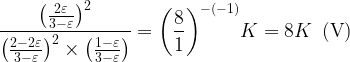
We can now establish the value of

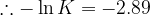
Resolving the logarithm,

Substituting in equation (V) yields

As before, we can solve the ensuing equation with Mathematica’s Solve command,
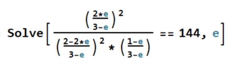
This returns two imaginary solutions and
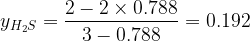
The sum of molar fractions is

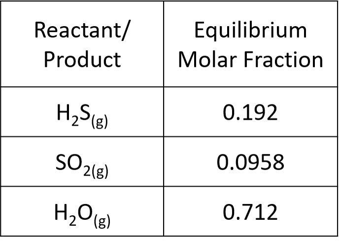
as one would expect. The results are summarized below.
Reference
• SMITH, J., VAN NESS, H. and ABBOTT, M. (2004). Introduction to Chemical Engineering Thermodynamics. 7th edition. New York: McGraw-Hill.