Capacity and Level of Service in Basic Freeway Segments

In this post, we analyze basic freeway segments in consonance with the method proposed in the Highway Capacity Manual. We begin by presenting an equation for the calculation of free-flow speed. We then propose an expression for analysis flow rate and briefly explain the meaning of each term. In the third section, we introduce the concept of level of service. Lastly, we present three solved examples.

Free-flow speed

The free-flow speed of a facility is best determined by field measurement. Given the shape of speed-flow relationships for freeways and multilane highways, an average speed measured when flow is less than or equal to 1,000 veh/h/ln may be taken to represent the free-flow speed.

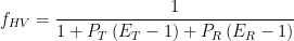
When field measurements are not possible, empirical formulas may be used. The free-flow speed of a freeway segment may be estimated with the expression

where is the adjustment for lane width (mi/h), is the adjustment for right-side lateral clearance (mi/h), and TRD is the total ramp density (ramps/mi). These terms are briefly described below.

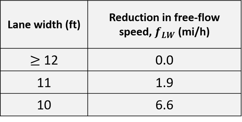
Lane width adjustment. The base condition for lane width is an average width of 12 feet or greater. For narrower lanes, the base free-flow speed is reduced in accordance with the following table.

Table 1. Adjustment to free-flow speed for lane width on a freeway

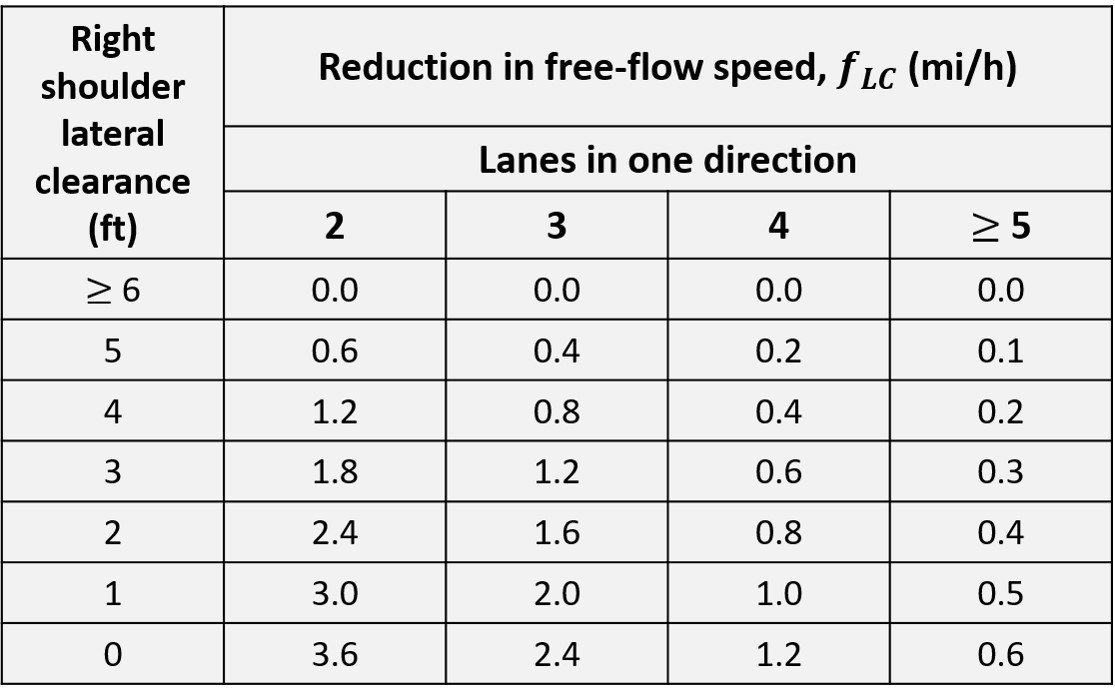
Lateral clearance adjustment. Base lateral clearance is 6 feet or greater on the right side and 2 feet or greater on the median, or left, side of the basic freeway section. Adjustments for right-side lateral clearances less than 6 feet are given in the following table.

Table 2. Adjustment to free-flow speed for lateral clearance on a freeway

Total ramp density adjustment. Ramp density provides a measure of the impact of merging and diverging traffic on free-flow speed. Total ramp density is the number of on- and off-ramps (in one direction) within a distance of three miles upstream and three miles downstream of the midpoint of the analysis segment, divided by six miles.

Analysis flow rate

The analysis flow rate is calculated using the following equation:

where is the 15-min passenger car flow rate (passenger car/hour/lane), V is the hourly volume (veh/h), PHF is the peak-hour factor, N is the number of lanes, is the heavy-vehicle adjustment factor, and is the driver population factor. The adjustment factors PHF, , and are briefly introduced next.

Peak-hour factor. Vehicle arrivals during the period of analysis [typically the highest hourly volume within a 24-hour period (peak hour)] will likely be nonuniform. To account for this varying arrival rate, the peak 15-min vehicle arrival rate within the analysis hour is usually used for practical traffic analysis purposes. The peak factor has been devised for this purpose, and is defined as the ratio of the hourly volume to the maximum 15-min flow rate expanded to an hourly volume. In mathematical terms,

where is the hourly volume for hour of analysis and is the maximum 15-min volume within hour of analysis. Factor 4 is of course the number of 15-min periods within an hour.

Heavy-vehicle factor. The most important adjustment to demand volume is the heavy-vehicle factor, which modifies for the presence of heavy vehicles in the traffic stream. A heavy vehicle is defined as any vehicle with more than four tires touching the pavement during normal operation. Two categories of heavy vehicles are used: (1) trucks and buses and (2) recreational vehicles (RVs). The heavy-vehicle adjustment factor is based on the principle of passenger car equivalents. A passenger car equivalent is the number of passenger cars displaced by one truck, bus, or RV in a given traffic stream under prevailing conditions. Given that two categories of heavy vehicle are used, two passenger car equivalents are used, namely , the passenger-car equivalent for trucks and buses, and , the passenger-car equivalent for RVs in the traffic stream under prevailing conditions. These factors are incorporated into the heavy-vehicle factor , which is expressed as

where is the proportion of trucks and buses and is the proportion of recreational vehicles in the traffic stream.

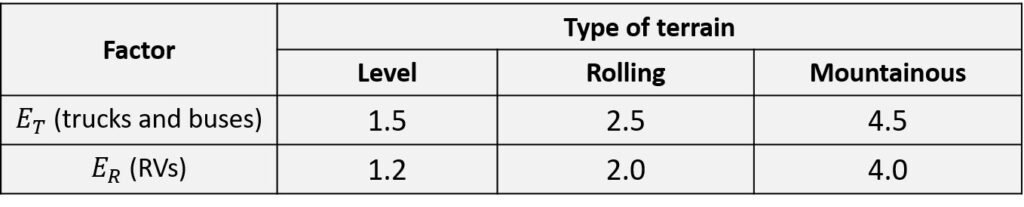
The Highway Capacity Manual specifies passenger-car equivalents for trucks and buses and RVs for extended sections of roadway in general terrain categories and for specific grade sections of significant impact. The general terrain sections are divided into three general categories: (1) level terrain, which consists of a combination of horizontal and vertical alignment permitting heavy vehicles to maintain approximately the same speed as passenger cars; (2) rolling terrain, any combination of horizontal and vertical alignment that causes heavy vehicles to reduce their speed but does not cause heavy vehicles to operate at their limiting speed; and (3) mountainous terrain, any combination of horizontal and vertical alignment that causes heavy vehicles to operate at their limiting speed for significant distances or at frequent intervals. The passenger-car equivalent factors can be taken from the following table.

Table 3. Passenger car equivalents for extended freeway segments

Driver population factor. Under base conditions, the traffic stream is assumed to consist of regular weekday drivers and commuters. Such drivers have a high familiarity with the roadway and generally maneuver and respond to the maneuvers of other drivers in a safe and predictable fashion. There are times, however, when the driver population has a driver population that is less familiar with the roadway in question (such as weekend drivers or recreational drivers). Such drivers can cause a significant reduction in roadway capacity relatively to the base condition of having only familiar drivers. To account for the composition of the driver population, the adjustment factor is used, and its recommended range is 0.85 – 1.0. Normally, the analyst should select a value of 1.0 for primarily commuter (or familiar-driver) traffic stream, but the value can be reduced from 1 to 15% for other driver populations.

Level of service

Traditionally, level of service (LOS) is a tool that assigns a letter grade on an A to F scale based on the quality of transportation as defined by various measurements, including estimates of speed, volume-to-capacity ratio, stops, or other criteria. The concept was first introduced in traffic analysis by the 1965 edition of the Highway Capacity Manual. The following table provides the level-of-service criteria corresponding to traffic density, speed, volume-to-capacity ratio, and maximum flow rate. A graphical representation of this table is provided in Figure 1. It should be borne in mind that, although parameters such as average speed and volume-to-capacity ratio are valuable parameters in traffic analysis, the primary determinant of LOS is density.

Table 4. LOS criteria for basic freeway segments

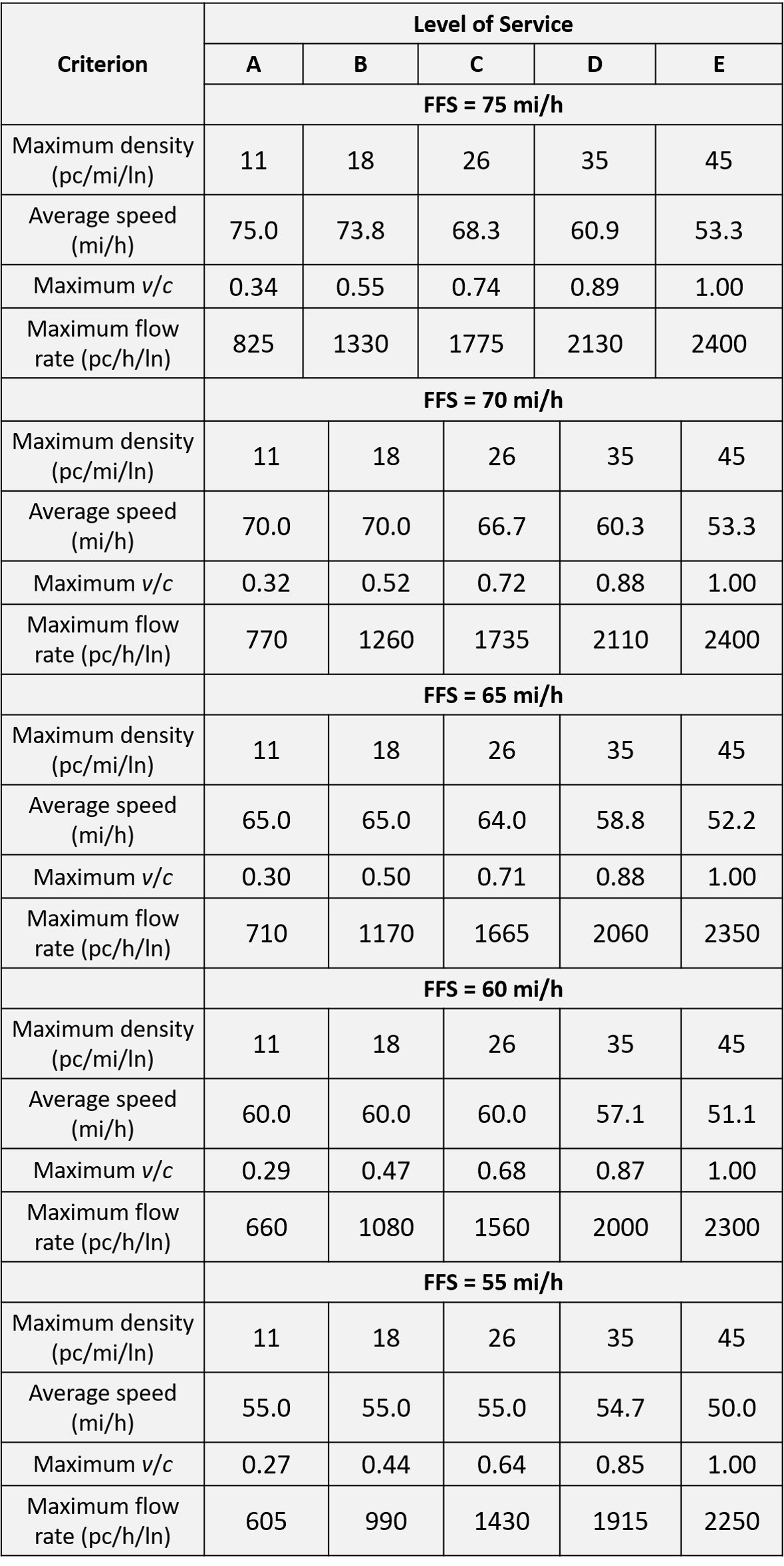
Figure 1. Basic freeway segment speed-flow curves and level-of-service criteria

Having presented an equation for free-flow speed, proposed an expression to calculate the analysis flow rate, and introduced the concept of level of service, we now turn to three simple solved problems.

Example 1

A six-lane urban freeway (three lanes in each direction) is on mountainous terrain with 10-ft lanes, obstructions 3 ft from the right edge of the traveled pavement, and ten ramps within three miles upstream and three miles downstream of the midpoint of the analysis segment. The traffic stream consists primarily of commuters. A directional weekday peak-hour volume of 2500 vehicles is observed, with 700 vehicles arriving in the most congested 15-min period. If the traffic stream has 12% large trucks and buses and no recreational vehicles, determine the level of service.

Since the lanes have a width of 10 ft, we read = 6.6 from Table 1. Given the right shoulder lateral clearance of 3 ft and the fact that there are 3 lanes in each direction, we read = 1.2 from Table 2.  The total ramp density is 10/3 = 3.33 ramps/mi. Substituting into equation (I), we obtain

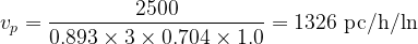
Rounding this result to the nearest 5 mi/h gives a FFS of 60 mi/h. The flow rate follows from equation (II), namely

The peak-hour factor is 2500/(700 4) = 0.893 and the number of lanes in each direction is N = 3. Lastly, the driving population factor is taken as 1. For mountainous terrain, = 4.5 (Table 3). Substituting in the heavy-vehicle adjustment factor equation gives

The flow rate is then

Entering this flow rate and a FFS of 60 mi/h into Figure 1, we read a speed S of 60 mi/h. The average speed is the same as the FFS because the flow rate is low enough such that it is still on the flat part of the speed-flow curve. Now, the density D is determined as

Referring to Table 4, we see that, for a density 18 D 26 and a maximum flow rate 1080 v  1560, the LOS is C. Accordingly, we conclude that this freeway segment operates at a level of service C.

Example 2

A freeway is being designed for a location in mountainous terrain. The expected free-flow speed is 55 mi/h. Lane widths will be 12 ft and shoulder widths will be 6 ft. During the peak hour, it is expected that there will be a directional peak-hour volume of 2700 vehicles, of which there are 12% buses and 6% recreational vehicles. The PHF and driver population adjustment are expected to be 0.88 and 0.90, respectively. If a level of service no worse than D is desired, determine the necessary number of lanes.

To begin, we compute the heavy-vehicle adjustment factor. From Table 3, we have, for mountainous terrain, = 4.5 and = 4.0. Accordingly,

Now, with reference to Table 4, the flow rate for the level of service to be no lower than D must not exceed 1915 pc/h/ln. Thus, appealing to equation (II) and setting = 1915 pc/h/ln, we can solve for the number of lanes N,

Rounding up to the nearest integer, we have N = 3. That is, if we are to have a level of service no worse than D, a six-lane freeway (three lanes in each direction) must be provided.

Example 3

A four-lane freeway (two lanes in each direction) is located on rolling terrain and has 11-ft lanes, a right-shoulder lateral clearance of 4 ft, and there are two ramps within three miles upstream of the segment midpoint and three ramps within three miles downstream of the segment midpoint. The traffic stream consists of cars, buses, and large trucks (no recreational vehicles). A weekday directional peak-hour volume of 1800 vehicles (familiar users) is observed, with 700 arriving in the most congested 15-min period. If a level of service no worse than C is desired, determine the maximum number of large trucks and buses that can be present in the peak-hour traffic stream.

The adjustment for lane width is = 1.9 (Table 1) and the lateral clearance adjustment is = 1.2. (Table 2). The ramp density is 2/6 = 0.333 ramps/mi, so that

Rounding to the nearest 5 mi/h, we surmise that FFS = 70 mi/h. The peak-hour factor is PHF = 1800/(700 4) = 0.643, the number of lanes in each direction is N = 2, and, for familiar drivers, = 1.0. From Table 3, the flow rate required for the level of service to be no lower than C is 1735 veh/h. Substituting these data into equation (II) brings to

But the proportion of special vehicles is given by equation (IV),

For rolling terrain, = 2.5 and = 2.0 (Table 3). Substituting and solving for ,

Lastly, the maximum number of trucks and buses is calculated as

In order for the level of service to be no lower than C, the number of trucks and buses in the traffic mix should be no greater than about 290 vehicles.

Go further

Montogue offers a full set of solved problems on highway capacity and level of service, which you can find here. Students of transportation engineering may also be interested in our quizzes on geometric design and analysis of signalized intersections. Check them out!

References

• Institute of Transportation Engineers. (2016). Traffic Engineering Handbook. 7th edition. Hoboken: John Wiley and Sons.

• MANNERING, F. and WASHBURN, S. (2013). Principles of Highway Engineering and Traffic Analysis. 5th edition. Hoboken: John Wiley and Sons.

• ROESS, R., PRASSAS, E. and MCSHANE, W. (2011). Traffic Engineering. 4th edition. Upper Saddle River: Pearson.