The curve number method was developed in the 1960s by the USDA Soil Conservation Service (SCS, now the Natural Resources Conservation Service), and has since established itself as a popular, ubiquitous, and enduring means of estimating storm runoff from rainfall events. In this article, we discuss the theory that underpins this method. To begin, let’s derive the basic precipitation-runoff relationship.
1. Development of the basic equation
The formulation of the SCS-CN method begins with the water budget expression, stated in depth units,

That is, rainfall (P) is runoff (Q) plus losses (F). We also require the potential maximum retention (or infiltration), S. The ratio of actual losses to potential losses can be assumed to be


Substituting 

This is the basic form of the runoff equation, and contains both rainfall (

However, internal agency review suggested that, for individual events, some amount of rainfall was required before runoff begins. This led to the introduction of the additional term 

The equation above applies so long as 


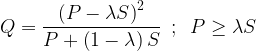
Studies were conducted and 

This is the commonly used form of the SCS-CN method.
2. The curve number CN
The parameter S representing the potential maximum retention depends on the soil-vegetation-land use complex of the catchment and also upon the antecedent soil moisture condition in the catchment just prior to the commencement of the rainfall event. This variable is expressed in terms of a dimensionless parameter CN, known as the curve number, in accordance with the relation

Alternatively, we can solve for CN and write
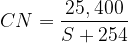
The curve number CN varies from zero to 100. A CN value of 100 represents a condition of zero potential retention (i.e., an impervious catchment), and CN = 0 represents an infinitely abstracting catchment with S = 
3. CN and soil types
CNs are strongly correlated to soil type. Soils have been divided into so-called Hydrologic Soil Groups (HSGs), whereby a given type of land is assigned to one of four categories (A, B, C, or D) depending on its hydrologic behavior. In one extreme, a letter A is attributed to to the most porous, deepest, and least runoff-prone ground, while, on the other extreme, a letter D is given to the shallowest, fine-textured, and most runoff-prone land. Each type is briefly described below.
Group A. These soils have low runoff potential and high infiltration rates even when thoroughly wetted. They consist mainly of deep, well to excessively drained sand or gravel and have a high rate of water transmission (greater than 0.30 in./hr).
Group B. These soils have moderate infiltration rates when thoroughly wetted and consist chiefly of deep to moderately well-drained soils with moderately fine to moderately coarse textures. This type of ground has a moderate rate of water transmission (0.15 – 0.30 in./hr).
Group C. These soils have low infiltration rates when thoroughly wetted, and consist chiefly of soils with a layer that impedes downward movement of water and soils with moderately fine to fine texture. This type of ground has a low rate of water transmission (0.05 to 0.15 in./hr).
Group D. These are soils with particularly high runoff potential. They have very low infiltration rates when thoroughly wetted and consist chiefly of clay soils with a high swelling potential, soils with a high permanent water table, soils with a claypan or clay layer at or near the surface, and shallow soils over nearly impervious material. This type of ground has a very low rate of water transmission.
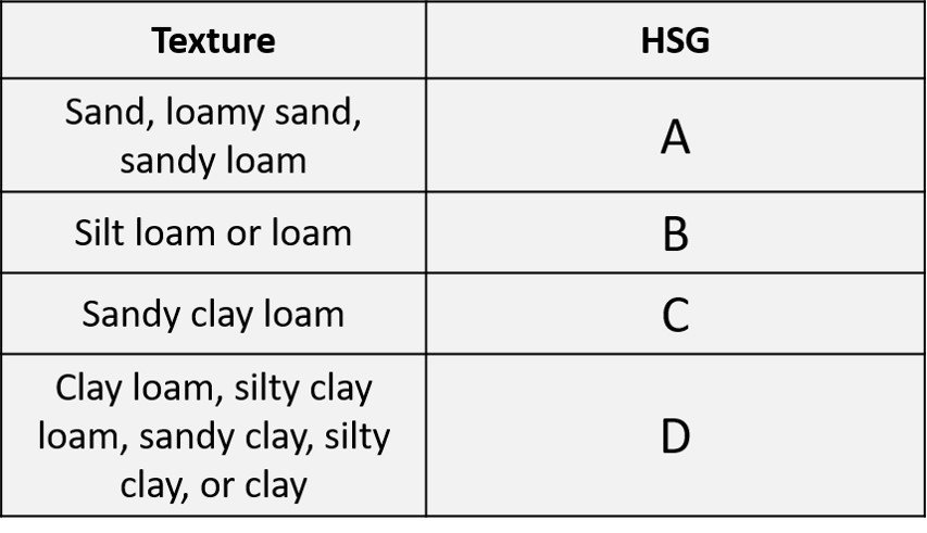
A SCS report published after the initial CN method paper gives simpler criteria, establishing HSG’s on the basis of soil texture only, as shown below.
Table 1. HSG’s based on soil texture
4. Antecedent moisture condition (AMC)
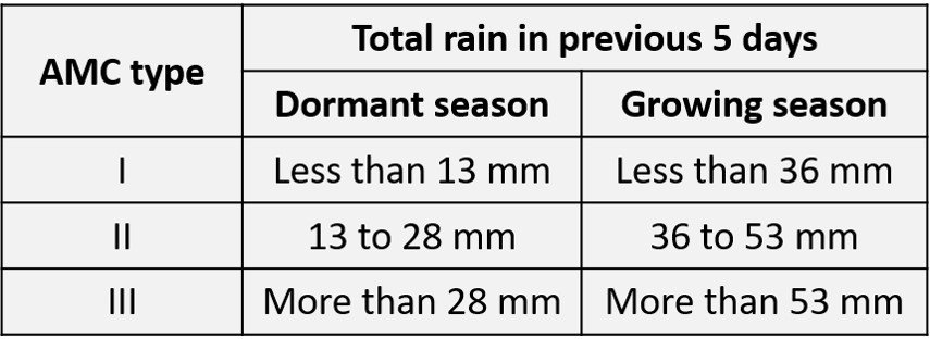
Antecedent moisture condition (AMC) refers to the moisture content present in the soil at the beginning of the rainfall-runoff event under consideration. It is well known that initial abstraction and infiltration are governed by AMC. For purposes of practical application, three levels of AMC are recognized in the SCS-CN method, and are established on the basis of the total rain in the previous 5 days, as listed below.
Table 2. Soil AMC categories
5. Land use and tabulated values of CN
The typical curve numbers for different types of land use, based on an AMC-II, are listed below.
Table 3. Curve numbers for different types of agricultural land use
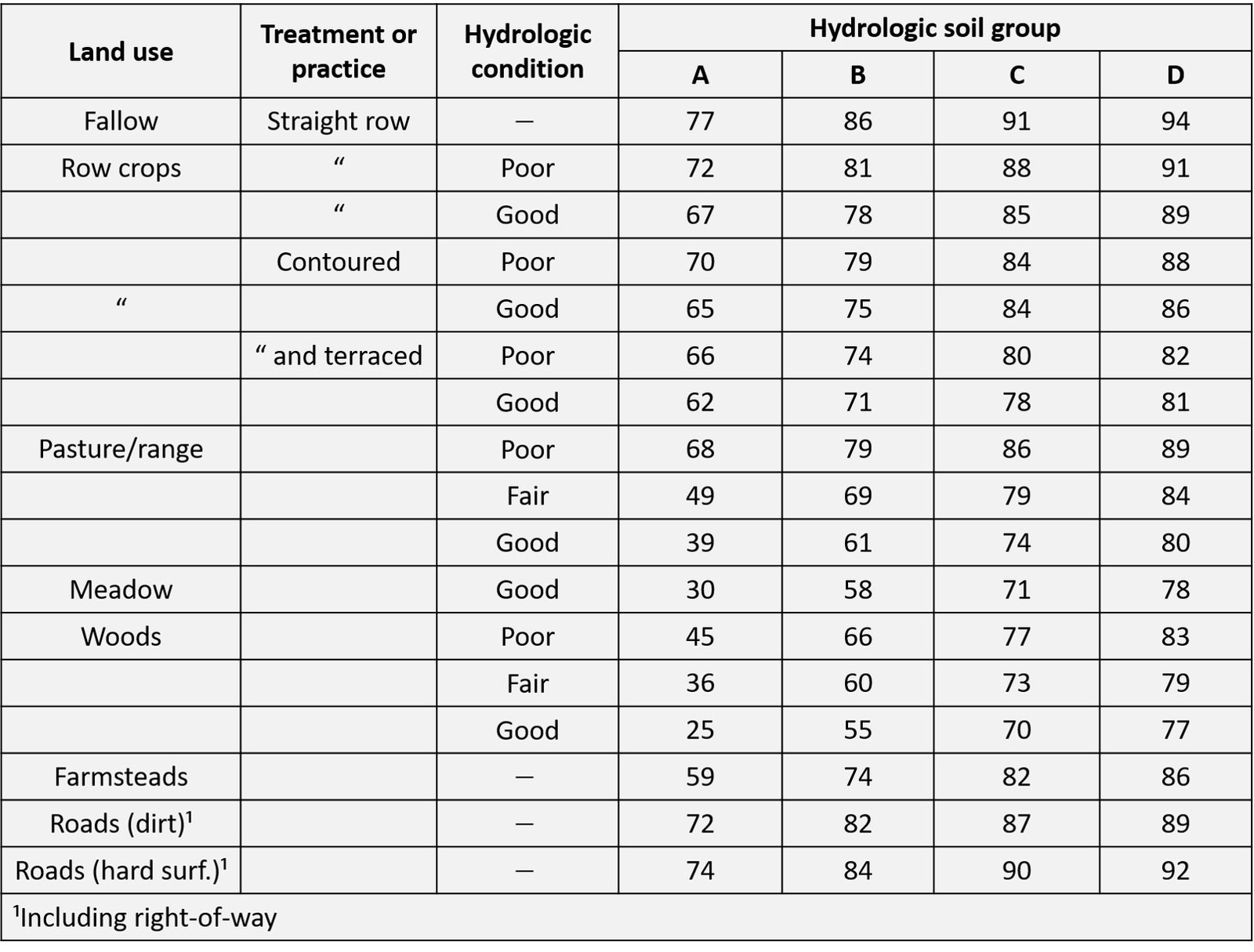
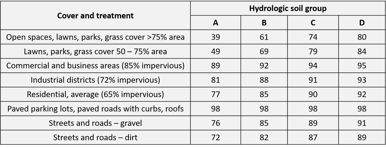
Note that the data above mainly involve terrains associated with agricultural practice, such as crops and pastures. Chow’s classic textbook Applied Hydrology contains data for surfaces associated with urban areas. As before, the data pertain to AMC-II conditions.
Table 4. Curve numbers for different types of urban land use
The curve numbers gleaned from the two previous tables can be converted to AMC-I and AMC-III values by dint of the following correlations:


To close this article, we present a simple example.
Example
A 400 ha watershed has been vigorously urbanized in recent years, and consists of 50% residential, 30% commercial/business areas, and 20% pure grass.
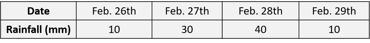
A) Estimate the value of direct runoff volume for the following 4 days of rainfall. The soil is a silt loam, and the AMC on February 26th was of category II.
B) What would the runoff volume be if the soil were categorized as AMC-III?
According to Table 1, a silt loam is associated with hydrologic soil group B. Curve numbers are taken from Table 4 and weighted in accordance with the percentage of cover that they represent, as shown in the following table.
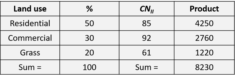
The average 

and the corresponding value of S is
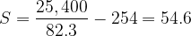
Accordingly, the runoff depth is described by the equation

which holds for P > 10.9 mm, otherwise the runoff is zero. The runoff values are computed in the following table.
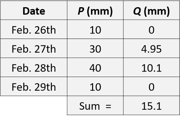
Lastly, the runoff volume is calculated as

Suppose now the soil belonged to AMC-III. In this case, the weighted 

The updated value of S is
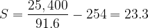
and the runoff depth is now described by the relation

This holds for P > 4.66 mm, otherwise the runoff is zero. The runoff values are computed below.
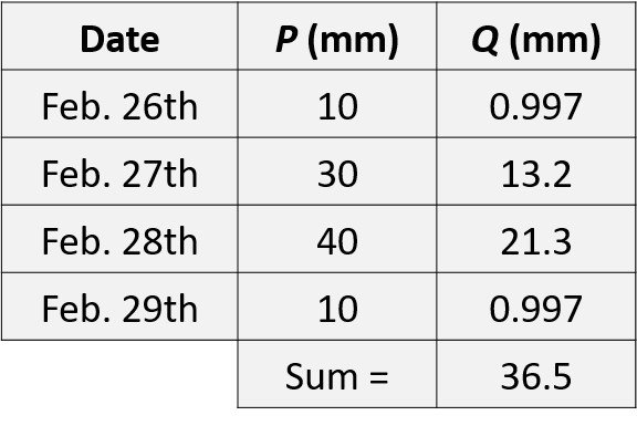
Finally, the runoff volume is calculated as

References
• CHOW, V., MAIDMENT, D. and MAYS, L. (1988). Applied Hydrology. New York: McGraw-Hill.
• HAWKINS, R., WARD, T., WOODWARD, D. and VAN MULLEM, J. (2009). Curve Number Hydrology: State of the Practice. Reston: ASCE Press.
• SUBRAMANYA, K. (2008). Engineering Hydrology. 3rd edition. New Delhi: Tata-McGraw-Hill.