Cooperative Game Theory: Core and Shapley Value

1. Transferable utility games

Economic agents can join forces and form coalitions that create value beyond that which a single agent or a smaller coalition could achieve on their own. The assumption is made that this value – often understood in units of utility or money – can be transferred at a one-to-one rate among any two players; this is the basis for a transferable utility coalitional game, or TU game for short. A TU game is a pair  = (N,v) where N = {1, 2, …, n} is a finite set of players and v: 2^N R is a coalitional or characteristic function that assigns to each coalition of players S  N a real number v(S) known as the worth of coalition S. The set N, that is, the set of all players, is often called the grand coalition.

The set of players N is obvious enough, but some students  struggle to understand the meaning of characteristic function v(S). In simple terms, the meaning of v(S) is that if the members of S agree to form this coalition, they can produce (or expect to receive) an amount v(S) of units of money, independently of the actions of the players who are not members of S.

There exist several subtypes of TU games, and the literature has a plethora of axioms and definitions with which to characterize them. Here’s one important definition:

Definition 1: Coalition Structure. A coalition structure CS = {C¹,C², …, C^k} is a partition of the player set N into mutually disjoint coalitions, that is,

Simply put, a coalition structure is basically a nonoverlapping partition of the player set. Next, we define two types of games:

Definition 2: Superadditive game. A TU game  = (N,v) is superadditive if for all coalitions S, T  N, if S  T = , then v(S  T)  v(S) + v(T).

Superadditivity is justified when coalitions can always work without interfering with one another, so that the value of two coalitions will be no less than the sum of their individual values. It also implies that there is a natural incentive for the coalition to form: for example, take a superadditive four-player game such that v({1,2}) = 3, v({3,4}) = 5, and v({1,2,3,4}) = 10. (Assume that there may be other characteristic function values for other coalitions.) The coalition with players 1 and 2 has 3 units of money, while the coalition with players 3 and 4 has 5; if the four players were to cooperate and form coalition S = {1,2,3,4}, they could obtain 10 units, which, since this game is superadditive, is at least as much as what the smaller coalitions could obtain on their own.

Lastly, note that superadditivity also implies that the grand coalition has the highest worth among all coalition structures.

Definition 3: Convex game. A TU game  = (N,v) is convex if for all coalitions S, T  N, if S  T = , then v(S  T)  v(S) + v(T) – v(S  T).

Note that convexity is a more restrictive condition than superadditivity. We mention convex games because they have desirable properties concerning the core and Shapley value, which we briefly discuss in sections 2 and 3, respectively.

2. The core

Definitions 4 and 5: Imputation and Core. Let  = {N,v} be a coalitional superadditive game. A candidate solution for this game is called an imputation (v), that is, an N-vector of real numbers (payoffs) x₁, x₂, …, x_N such that

As stated, an imputation is a set of imputed payoffs that satisfy two requirements. The expression to the left indicates that imputations are efficient, as their components add up to the worth of the grand coalition, v(N). The expression to the right indicates that imputations satisfy individual rationality, as no player benefits from quitting the grand coalition and playing alone. Equipped with the definition of imputation, we press on to define the core as the set of payoffs given by

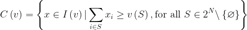
A payoff is in the core if and only if the sum of payoffs to any group of players S  N is as large as the payoffs that these players could share among themselves if they broke away and formed a coalition of their own. As shown in the formula, all payoff vectors in the core are also imputations.

If C(v) , then elements of the core can be easily obtained with the aid of a finite system of linear inequalities. Solving the inequalities that describe a core is a process akin to linear programming, a maximization/minimization technique that should be familiar to those who have taken a basic optimization course.

Leyton-Brown and Shoham (2008) note that, since the core provides a notion of stability for coalitional games, we can regard it as somewhat of an analog of the Nash equilibrium in noncooperative game theory. Payoffs in a core are such that the players in the coalition that receives them cannot gain more by unilaterally breaking away or forming a different subcoalition, much like an agent in a two-player static game cannot do better by unilaterally deviating from a Nash equilibrium. That said, this comparison doesn’t really do justice to the core, however, because the latter reflects stability for a whole set of subcoalitions of players, whereas the Nash equilibrium describes stability only with respect to deviation by a single agent. The core is generally a more stringent solution concept than the Nash equilibrium.

A TU game’s core can be empty, which is perhaps its main limitation. When attempting to find and characterize a core, the modeler may want to establish in advance whether the problem lends itself to the use of this solution concept at all. One great place to start is to check whether the game is a convex game, because:

Theorem. Every convex game has a nonempty core.

For more general games, one may resort to the Shapley-Bondareva theorem, which is closely related to the concept of balancedness. Before stating the theorem, we need a few more definitions.

Definition 6: Indicator function. Given a set S N, we denote : N  {0,1} as the indicator function of the set S, that is, let (i) = 1 if i  S and $latex \displaystyle {{\chi }_{S}}(i) = 0$ if i N\S.

Definitions 7 and 8: Balanced collection; Balancing weight system. A collection of sets B  2^N\{} is said to be balanced if there exists a vector  of positive numbers such that

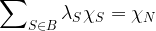
The vector is called the balancing weight system for B. The interpretation of the concept of a balanced weight system is that it is a rule expressing the portion of unitary time that a player dedicates to each coalition S to which he belongs.

Here’s the theorem itself:

Theorem (Bondareva-Shapley). A superadditive TU game  = (N,v) has a non-empty core if an only if for every balanced collection B  2^N\{} and any balanced weight system  for B it holds that

While the Bondareva-Shapley theorem may be used to ascertain whether a core is in fact empty, it is not very efficient since the number of balanced set systems is superexponential in the number of players N.

3. Shapley value

The Shapley value was introduced in 1951 by Lloyd S. Shapley, who was awarded the 2012 Nobel Prize in economics for it. Whereas the core belongs to the domain of coalitional stability, the Shapley value is an attempt to model the coalition members’ marginal contribution to some cooperative endeavor and distribute the coalition’s worth with fairness.

It is often implicitly assumed that the games to which the Shapley value is applied are superadditive (recall that in superadditive games it makes sense for the grand coalition to form). Shapley’s 1951 and 1953 papers referred to superadditive games because, a few years earlier, von Neumann and Morgenstern (1944) had relied on this assumption as part of their treatment of cooperative games in The Theory of Games and Economic Behavior. It should be noted, however, that the Shapley value holds for any TU game, superadditive or not.

The Shapley value associated with player i may be defined as

In contrast to the core, which may be empty and somewhat hard to compute, the Shapley value is always well-defined and given by an explicit formula.

A number of authors have proposed various ways to interpret and calculate the Shapley value, but the most intuitive one continues to be the ‘bargaining model’ approach due to Shapley himself. In this reasoning, he noted that the grand coalition can be formed in such a way that all the players would be admitted one by one until everyone was included and the grand coalition was formed. Upon entering, each player would introduce a marginal contribution to the coalition’s worth relatively to the coalition that preceded the player’s adherence. The order of entrance would be randomly selected with all orderings being equally probable. The contributions would be added and normalized by the number of permutations, leading to a ‘fair’ payoff to each player.

Arguably, the main limitation of the Shapley value is that it does not always appear in the core. For convex games, however, we can safely say that:

Theorem. In every convex game, the Shapley value is in the core.

Example

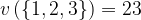
Consider the three-player game whose characteristic function satisfies

The marginal contributions to each player’s Shapley value are tabulated below.

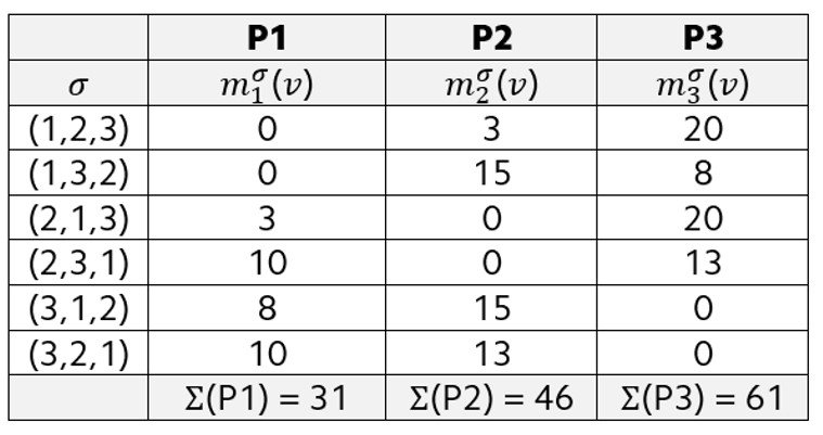
To see how the calculations work, refer to the first entry, in which we have the permutation (1,2,3); needless to say, in this permutation player 1 enters first, player 2 enters second, and player 3 enters third. Column P1 lists the marginal contribution associated with player 1; for the (1,2,3) permutation, player 1’s contribution is zero because player 1 enters first and v({1}) = 0. Column P2 lists the marginal contribution associated with player 2; for the (1,2,3) permutation, player 2’s contribution is 3 because player 2 enters after player 1 is already there, so we have v({1,2}) – v({1}) = 3 – 0 = 3. Column P3 lists the marginal contribution associated with player 3; for the (1,2,3) permutation, player 3’s contribution is 20 because player 3 enters after players 1 and 2 are already there, so we have v({1,2,3}) – v({1,2}) = 23 – 3 = 20.

Consider the second entry, in which we have permutation (1,3,2); in this case player 1 enters first, player 3 enters second, and player 2 enters third. Column P1 lists the marginal contribution associated with player 1; for the (1,3,2) permutation, player 1’s contribution is zero because player 1 enters first and v({1}) = 0. Column P2 lists the marginal contribution associated with player 2; for the (1,3,2) permutation, player 2’s contribution is 15 because player 2 enters after players 1 and 3 are already there, so we have v({1,2,3}) – v({1,3}) = 23 – 8 = 15. Column P3 lists the marginal contribution associated with player 3; for the (1,2,3) permutation, player 3’s contribution is 8 because player 3 enters after player 1 is already there, so we have v({1,3}) – v({1}) = 8 – 0 = 8.

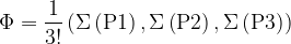
Calculations for other row entries are analogous. After all permutations have been accounted for, we add the rows for each player and divide the result by 3! = 6 to obtain the players’ Shapley value components; in the present case:

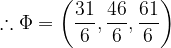
As a useful check, note that the sum of the players’ Shapley values should equal the worth of the grand coalition:

References

• BAUSO, D. (2016). Game Theory with Engineering Applications. Society for Industrial and Applied Mathematics.

• CHALKIADAKIS, G., ELKIND, E. and WOOLDRIDGE, M. (2012). Computational Aspects of Cooperative Game Theory. Morgan and Claypool Publishers.

• LEYTON-BROWN, K. and SHOHAM, Y. (2008). Essentials of Game Theory. Morgan and Claypool Publishers.

• VON NEUMANN, J. and MORGENSTERN, O. (1944). The Theory of Games and Economic Behavior. Princeton University Press.