Yager’s Ordered Weighted Averaging Operators

1. Defining the OWA operator

Averaging is the most common way to combine inputs. It is commonly used in a series of quotidian applications, such as multicriteria decision making, voting, and performance scores. The basic rule shared by all averaging functions is that the total score cannot be above or below any of the inputs (Beliakov et al., 2007). The aggregated value is seen as some sort of representative value of all the inputs.

Ordered weighted averaging (OWA) operators were first proposed by Yager in 1988. As the name implies, the OWA operator takes in a set of conveniently ordered numbers and a vector of weights, and then returns an aggregated value. In introducing the OWA operator, Yager drew on the notion that T-norms and T-conorms represent aggregation operators that generalize the notion of conjunction and disjunction of classical logic with, in particular, the min operator being the maximal T-norm and the max operator being the minimal T-conorm. OWA operators satisfy the property of filling the gap between min and max operators in a continuous manner (Cutello and Montero, 1995) – a desirable trait for fuzzy system applications, which were the focus of Yager’s work.

Let a_i, i = 1, 2, 3, …, n be a collection of n numbers, known as arguments, and an associated weighing vector W = {w₁, w₂, w₃, …, w_n} of dimension n such that $\displaystyle \Sigma$ w_j = 1, j = 1, 2, …, n. The ordered weighted averaging operator of dimension n is a mapping F: $\displaystyle {{\mathbb{R}}^{n}}$ $\displaystyle \to$ $\displaystyle \mathbb{R}$ defined by

$\displaystyle \text{OWA}\left( {{{a}_{1}},{{a}_{2}},{{a}_{3}},...,{{a}_{n}}} \right)=\sum\limits_{{j=1}}^{n}{{{{w}_{j}}{{b}_{j}}}}\,\,\,(1)$

where (b₁, b₂, b₃, …, b_n) is a permutation of (a₁, a₂, a₃, …, a_n) where arguments are ordered from largest to smallest. That is, b_j is the j-th largest element in a_i.

As can be seen, the formula used to compute the OWA is quite simple and can be readily applied in hand calculations or, in the case of large datasets, implemented in code. As an example, suppose we have the dataset a = (1, 5, 3, 9, 7) and the weight vector w = (0.25, 0.1, 0.1, 0.35, 0.2). Note first that the weights in vector w add up to one, as they should. Before applying equation (1), we need to rearrange the a_i’s in decreasing order, that is:

$\displaystyle a=\left( {1,5,3,9,7} \right)\to b=(9,7,5,3,1)$

Finally,

$\displaystyle \text{OWA}\left( a \right)=9\times 0.25+7\times 0.1+5\times 0.1+3\times 0.35+1\times 0.2=4.7\leftarrow$

2. Properties and special cases

Several properties and special cases of the OWA operator have been reported in the literature, and some are immediately apparent. The most basic property is of course

$\displaystyle \min \left( {{{a}_{1}},...,{{a}_{n}}} \right)\le \text{OWA}\left( {{{a}_{1}},...,{{a}_{n}}} \right)\le \max \left( {{{a}_{1}},...,{{a}_{n}}} \right)\,\,\,;\,\,\,(2)$

That is, like every aggregating function, the OWA operator always returns a value that is no less than the smallest input and no greater than the greatest input.

Also, the OWA operator is symmetric, which means that, for some argument set (a₁, a₂, …, a_n) and any of its permutation maps (a_π(1), a_π(2), …, a_π(n)), the aggregated value returned by the operator is the same,

$\displaystyle \text{OWA}\left( {{{a}_{1}},...,{{a}_{n}}} \right)=\text{OWA}\left( {{{a}_{{\pi \left( 1 \right)}}},...,{{a}_{{\pi \left( n \right)}}}} \right)\,\,\,(3)$

This property becomes obvious if we note that it does not matter what the initial ordering of the input vector is, as the OWA calculation always involves rearranging the values from lowest to highest before we apply the weights (James, 2016).

As with all aggregating functions, the OWA is also monotone and idempotent:

$\displaystyle \text{OWA}\left( {{{a}_{1}},...,{{a}_{n}}} \right)\ge \text{OWA}\left( {{{q}_{1}},...,{{q}_{n}}} \right)\,\text{if }{{a}_{i}}\ge {{q}_{i}}\ \text{for}\,i=1,2,...,n\,\,\,(4)$

$\displaystyle \text{OWA}\left( {{{a}_{1}},...,{{a}_{n}}} \right)\,=a\,\,\text{if}\,{{a}_{1}}={{a}_{2}}=...={{a}_{n}}=a\,\,\,(5)$

Let the weighting vector be such that w₁ = 1 and w_j = 0 for j $\displaystyle \ne$ 1. The weighting vector in this case may be denoted as $\displaystyle {{W}^{*}}$ , and the operator returns

$\displaystyle \text{OWA}\left( {{{a}_{1}},{{a}_{2}},...,{{a}_{n}}} \right)=\max \left( {{{a}_{j}}} \right)\,\,\,(6)$

Thus, the max operator is a special case of the OWA operator. Similarly, if the weights are selected such that w_n = 1 and w_j = 0 for j $\displaystyle \ne$ n, the weighting vector may be denoted as $\displaystyle {{W}_{*}}$ and the operator returns

$\displaystyle \text{OWA}\left( {{{a}_{1}},{{a}_{2}},...,{{a}_{n}}} \right)=\min \left( {{{a}_{j}}} \right)\,\,\,(7)$

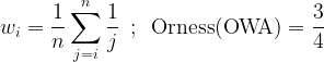
Thus, the min operator is also a special case of the OWA operator. Further, if the weights are assigned such that w_j = 1/n for all j, the weighting vector may be denoted as $\displaystyle {{W}_{{\text{ave}}}}$ and the operator becomes

$\displaystyle \text{OWA}\left( {{{a}_{1}},{{a}_{2}},...,{{a}_{n}}} \right)=\frac{1}{n}\sum\limits_{{j=1}}^{n}{{{{a}_{j}}}}\,\,\,(8)$

which is easily recognized as the arithmetic mean. Thus, the simple average is also a special case of the OWA operator.

The median is also a special case of the OWA operator. If n is odd we obtain the median by selecting w_(n+1)/2 = 1 and letting w_j = 0 for j $\displaystyle \ne$ (n+1)/2. If n is even we get the median by selecting w_n/2 = w_n/2+1 = 1/2 and letting w_j = 0 for all other terms.

Lastly, it can be shown that the OWA also generalizes the mode, the trimmed arithmetic mean, and the winsorized mean (Yager, 1997).

To every OWA with weighting vector w = (w₁, …, w_n-1, w_n) there corresponds a so-called reverse OWA with weighting vector w = (w_n, w_n-1, …, w₁). Properties of typical OWA operators also apply to reverse OWAs.

The OWA operator is akin to the well-known weighted mean operation, as both are linear combinations of the values (arguments) with respect to the weights. There are appreciable differences between the two operators, however; for one, while the OWA can model the minimum and the maximum operators, the weighted mean cannot; on the other hand, the weighted mean can be used to model dictatorship (the value of one of the sources is always selected), whereas OWA cannot.

The most striking differences in behavior between the weighted mean and the OWA operator arise when we consider the effect that the reordering of arguments – a feature of the OWA, but not of the weighted mean – has in practical terms. As noted by Torra and Narukawa (2007), the weighting vectors in the weighted mean are used to express the reliability of the information sources that have supplied a particular value, which is to say that each weight w_i corresponds to a measure of the reliability of the i-th sensor or the expertise of the i-th expert. This is not the case with the OWA operator, where the ordering of weights can reduce the importance of extreme values (or even ignore them) or give greater importance to small values rather than large ones. This essentially translates into weighting the values rather than weighting the sources. According to this interpretation, there are applications in which both techniques are useful, as the insights afforded by them may be complementary rather than exclusive.

3. Orness of an OWA operator

The concept of orness has been introduced to characterize aggregating functions in terms of how close, so to speak, to the maximum function they are. (Recall that, in fields such as fuzzy set theory, logical or is associated with the maximum operation, hence the name.) The maximum operator has an orness degree of 1, while the minimum operator has an orness degree of 0. The arithmetic mean, which treats high and low inputs equally, has an orness of 0.5. Importantly, while it is true that only an OWA with weighting vector $\displaystyle {{W}^{*}}$ (i.e., an OWA that becomes the max operator) can have an orness of 1 and only an OWA with weighting vector $\displaystyle {{W}_{*}}$ (i.e., an OWA that becomes the min operator) can have an orness of 0, infinitely many weighting vectors exist for orness values in between. For example, any OWA operator with a weighting vector such that w_n–j+1 = w_j has orness = 0.5.

Calculating the orness of an aggregating function is often a complicated process, involving multivariate integrations and other intricate techniques, but in the case of the OWA operator all we need is the weighting vector. Indeed, for a given weighting vector w = (w₁, w₂, w₃, …, w_n), the degree of orness of the associated OWA operator is given by

$\displaystyle \text{Orness}\left( w \right)=\sum\limits_{{i=1}}^{n}{{{{w}_{i}}\frac{{i-1}}{{n-1}}}}\,\,\,(9)$

Returning to the dataset introduced in section 1, we may compute the orness as follows. The multipliers for the weights are:

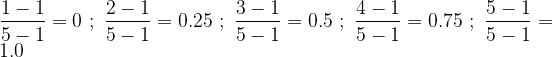
$\displaystyle \frac{{1-1}}{{5-1}}=0\,\,;\,\,\frac{{2-1}}{{5-1}}=0.25\,\,;\,\,\frac{{3-1}}{{5-1}}=0.5\,\,;\,\,\frac{{4-1}}{{5-1}}=0.75\,\,;\,\,\frac{{5-1}}{{5-1}}=1.0$

The corresponding orness is:

$\displaystyle \text{Orness}\left( a \right)=0.25\times 0+0.1\times 0.25+0.1\times 0.5+0.35\times 0.75+0.2\times 1.0=0.538\leftarrow$

The orness of a OWA operator has several properties of interest. For example, the orness of a OWA and its reverse (we’ve defined a reverse OWA above) are related by

$\displaystyle \text{Orness}\left( {\text{OWA}} \right)=1-\text{Orness}\left( {\text{OW}{{\text{A}}_{d}}} \right)\,\,\,(10)$

A self-dual OWA is such that its dual, that is, its corresponding reverse OWA has the same weighting vector as the OWA itself. Putting Orness(OWA) = Orness(OWA_d) in the equation above, we obtain

$\displaystyle \text{Orness}\left( {\text{OWA}} \right)=\frac{1}{2}$

which means that an OWA will be self-dual only if its orness equals 0.5. For example, the arithmetic mean OWA (equation (8)) is self-dual, as we’d expect. In addition, if the weighting vector is non-decreasing, i.e., w_i $\displaystyle \le$ w_i+1, i = 1, …, n – 1, it can be shown that the orness of the OWA will lie between 0.5 inclusive and 1 inclusive. Likewise, if the weighting vector is non-increasing, the orness of the OWA will lie between 0 inclusive and 0.5 inclusive.

If two OWA functions with weighting vectors w₁ and w₂ have respective orness values $\displaystyle {{O}_{1}}$ and $\displaystyle {{O}_{2}}$ , and the weighting vectors are related by

$\displaystyle {{\mathbf{w}}_{3}}=t{{\mathbf{w}}_{1}}+\left( {1-t} \right){{\mathbf{w}}_{2}}\,\,\,;\,\,\,t\in \left[ {0,1} \right]\,\,\,(11)$

then a OWA₃ with weighting vector w₃ will have orness value

$\displaystyle \text{Orness(OW}{{\text{A}}_{3}})=t{{O}_{1}}+\left( {1-t} \right){{O}_{2}}\,\,\,(12)$

Lastly, Beliakov et al. (2007) quote orness values for two special weighting vectors:

$\displaystyle {{w}_{i}}=\frac{1}{n}\sum\limits_{{j=i}}^{n}{{\frac{1}{j}\,\,\,;\,\,\,\text{Orness(OWA)}=\frac{3}{4}}}$

$\displaystyle {{w}_{i}}=\frac{{2\left( {n+1-i} \right)}}{{n\left( {n+1} \right)}}\,\,\,;\,\,\,\text{Orness}\left( {\text{OWA}} \right)=\frac{2}{3}$

Some authors (e.g., Cutello and Montero, 1995) also speak of measures of andness, which represent how close an operator is to the min operator. Andness is the dual of orness and can be related to it by the simple expression

$\displaystyle \text{Andness}\left( w \right)=1-\text{Orness}\left( w \right)\,\,\,(13)$

4. Induced ordered weighted averaging operators

The foregoing discussion makes clear that the most important step in the calculation of the OWA is the permutation of the input data according to the size of its arguments. Unfortunately, some applications require that, during the averaging process, inputs be sorted not necessarily in decreasing fashion but rather with reference to some other rule, perhaps a function of the values themselves. With this concept in mind, Yager and Filev (1999) introduced the induced weighted averaging (IOWA) operator. The induced OWA provides a more general framework for the reordering process, as an inducing variable can be defined, on either numerical or ordinal spaces, which then dictates the order by which the arguments are permuted.

Given a weighting vector w = (w₁, w₂, …, w_n) and an inducing variable z, the Induced Ordered Weighted Averaging (IOWA) function is

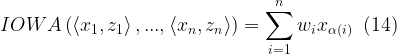
$\displaystyle IOWA\left( {\left\langle {{{x}_{1}},{{z}_{1}}} \right\rangle ,...,\left\langle {{{x}_{n}},{{z}_{n}}} \right\rangle } \right)=\sum\limits_{{i=1}}^{n}{{{{w}_{i}}{{x}_{{\alpha \left( i \right)}}}}}\,\,\,(14)$

where the $\displaystyle \alpha$ (۰) notation denotes the inputs 〈x_i, z_i〉 reordered such that z_α₍₁₎ z_α₍₂₎ … z_α_(n) and the convention that if q of the z_α_(i) are tied, i.e. z_α_(i) = z_α_(i+1) = … = z_α_(i+q-1), then

$\displaystyle {{x}_{{\alpha \left( i \right)}}}=\frac{1}{q}\sum\limits_{{j=\alpha \left( i \right)}}^{{\alpha \left( {i+q-1} \right)}}{{{{x}_{j}}}}\,\,\,(15)$

An inducing variable can be based on any notion that associates a variable with each input x_i. Where x_i provides information to be aggregated, z_i provides some information about x_i. The input pairs 〈x_i,z_i〉 may be two independent features of the same input, or can be related by some function, i.e., z_i = f_i(x_i). It is conventional for introducing variables used with the IOWA to permute z in non-decreasing order.

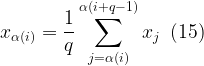
Suppose we had the weight vector w = (0.25, 0.1, 0.35, 0.3) and the input 〈x, z〉 = (〈1, 4〉, 〈3, 2〉, 〈5, 8〉, 〈7, 6〉). The aggregated value for the induced OWA is, in this case,

$\displaystyle \text{IOWA}\left( {\left\langle {x,z} \right\rangle } \right)=0.25\times 5+0.1\times 7+0.35\times 1+0.3\times 3=3.2\leftarrow$

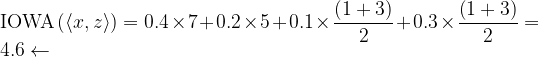
Suppose we had the weight vector w = (0.4, 0.2, 0.1, 0.3) and the input 〈x, z〉 = (〈1, 4〉, 〈3, 4〉, 〈5, 6〉, 〈7, 8〉). Note that there is a tie, z₁ = z₂ = 4, hence we must appeal to equation (15). The aggregated value for the induced OWA is then

$\displaystyle \text{IOWA}\left( {\left\langle {x,z} \right\rangle } \right)=0.4\times 7+0.2\times 5+0.1\times \frac{{\left( {1+3} \right)}}{2}+0.3\times \frac{{\left( {1+3} \right)}}{2}=4.6\leftarrow$

For a thorough review of the properties and applications of IOWA operators, see Beliakov and James (2011).

References

Beliakov, G. and James, S. (2011). Induced ordered weighted averaging operators. In: YAGER, R.R., KACPRZYK, J. and BELIAKOV, G. (Eds.). Recent Developments in the Ordered Weighted Averaging Operators: Theory and Practice. Berlin/Heidelberg: Springer.
BELIAKOV, G., PRADERA, A. and CALVO, T. (2007). Aggregation Functions: A Guide for Practicioners. Berlin/Heidelberg: Springer.
Cutello, V. and Montero, J. (1995). The computational problem of using OWA operators. In: BOUCHON-MEUNIER, B., YAGER, R.R. and ZADEH, L.A. (Eds.). Fuzzy Logic and Soft Computing. Singapore: World Scientific.
JAMES, S. (2016). An Introduction to Data Analysis using Aggregation Functions in R. Berlin/Heidelberg: Springer.
TORRA, V. and NARUKAWA, Y. (2007). Modelling Decisions: Information Fusion and Aggregation Operators. Berlin/Heidelberg: Springer.
Yager, R.R. (1997). On the inclusion of importances in OWA aggregation. In: YAGER, R.R. and KACPRZYK, J. (Eds.). The Ordered Weighted Averaging Operators. Berlin/Heidelberg: Springer.
Yager, R.R. and Filev, D.P. (1999). Induced ordered weighted averaging operators. IEEE Transactions on Systems, Man, and Cybernetics – Part B: Cybernetics, 20:2, 141 – 150.

Yager’s Ordered Weighted Averaging Operators

Subscribe to our Mailing List!

Featured Posts

A Primer on NAND Flash Memories

Solidification Time and Chvorinov’s Rule

Step-Growth Polymerization, the Carothers Equation, and the Flory-Schulz Distribution

More Articles

Fresnel Diffraction and the Cornu Spiral

RSA Public-Key Cryptography and Pollard’s p – 1 Factorization

Fields of Study

More

© 2024 Montogue Quiz

Subscribe to
our Mailing List!

Subscribe to our Mailing List!

Subscribe to receive our latest materials in your inbox.

Homework Help

© 2024 Montogue Quiz

Subscribe to our Mailing List!