Air Pollution and the Gaussian Plume Model

The Gaussian plume model predicts the concentration of an atmospheric emission, such as a gaseous pollutant or aerosol, downwind of a point source of release. A real system often modeled by this approach is the release of smoke by an industrial exhaust stack, although, in principle, any point source of gas with a fixed distance above ground can have its dispersion represented by a Gaussian plume. In this article, we provide a quick introduction to this elegant theory, including a quick discussion on each parameter involved (dispersion coefficients, wind speed) and a solved example.

1. Introducing the Gaussian plume

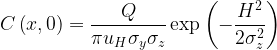
Referring to the illustration in Figure 1, the three-dimensional coordinate system we propose has the stack at the origin, with distance downwind given by x, distance off the downwind axis given by y, and elevation given by z. Since in most environmental applications we are only interested in ground-level concentrations, we set z = 0 and state the basic equation of the Gaussian plume model as

$\displaystyle C\left( {x,y} \right)=\frac{Q}{{\pi {{u}_{H}}{{\sigma }_{y}}{{\sigma }_{z}}}}\exp \left( {-\frac{{{{H}^{2}}}}{{2\sigma _{z}^{2}}}} \right)\exp \left( {-\frac{{{{y}^{2}}}}{{2\sigma _{y}^{2}}}} \right)$

where x is the distance directly downwind, y is the horizontal distance from the plume centerline, C is the concentration at (x,y), Q is the emission rate of pollutants, H is the effective stack height, u_H is the average wind speed at the effective height of the stack, $\displaystyle {{\sigma }_{y}}$ is the horizontal dispersion coefficient, and $\displaystyle {{\sigma }_{z}}$ is the vertical dispersion coefficient. This simple equation gives the time-averaged concentration of an air pollutant at any spatial location downwind of a source. The first term to the right of the equal sign provides the concentration directly at the centerline of the plume (coordinates x,0,0); the second term adjusts the concentration in the vertical (z) direction; the third term adjusts the concentration as we move in the sideways (y) direction.

Figure 1. Orientation of the Gaussian plume model.

The effective stack height H is given by the sum of physical stack height, h, and the plume rise, $\displaystyle \Delta$ h, i.e. H = h + $\displaystyle \Delta$ h. Plume rise is caused by a combination of factors, the most important ones being the buoyancy and momentum of the exhaust gases, and the stability of the atmosphere itself. Over the years, several approaches have been proposed for the calculation of plume rise, often with very different results. One historically important equation was proposed by Holland in 1953:

$\displaystyle \Delta h=\frac{{{{v}_{s}}d}}{{{{u}_{H}}}}\left\{ {1.5+\left[ {0.0268P\left( {\frac{{{{T}_{s}}-{{T}_{a}}}}{{{{T}_{s}}}}} \right)d} \right]} \right\}$

where v_s is stack velocity (m/s), d is stack diameter (m), u_H is wind speed (m/s), P is pressure (kPa), T_s is stack temperature (K) and T_a is air temperature (K).

Coefficients $\displaystyle {{\sigma }_{y}}$ and $\displaystyle {{\sigma }_{z}}$ are referred to as dispersion coefficients (or sometimes dispersion lengths). These parameters increase with downwind distance x, which means that the plume spreads farther away from the centerline and effective stack height. Accordingly, the maximum concentration of the air pollutant will occur along the plume’s centerline. Also, note how the Gaussian plume equation does not have an explicit term for x; instead, concentration decay of pollutant as we move away from the source is represented by increasing values of $\displaystyle {{\sigma }_{y}}$ and $\displaystyle {{\sigma }_{z}}$ .

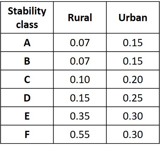
The values of $\displaystyle {{\sigma }_{y}}$ and $\displaystyle {{\sigma }_{z}}$ depend on atmospheric stability conditions, which are labeled A through F. The label A refers to very unstable atmospheric conditions, B to unstable conditions, C to slightly unstable conditions, D to neutral conditions, E to stable conditions, and F to very stable conditions. A key to classify atmospheric conditions as a function of parameters such as wind speed, solar radiation and sky cloudiness is given in Table 1.

Table 1. Atmospheric stability classification

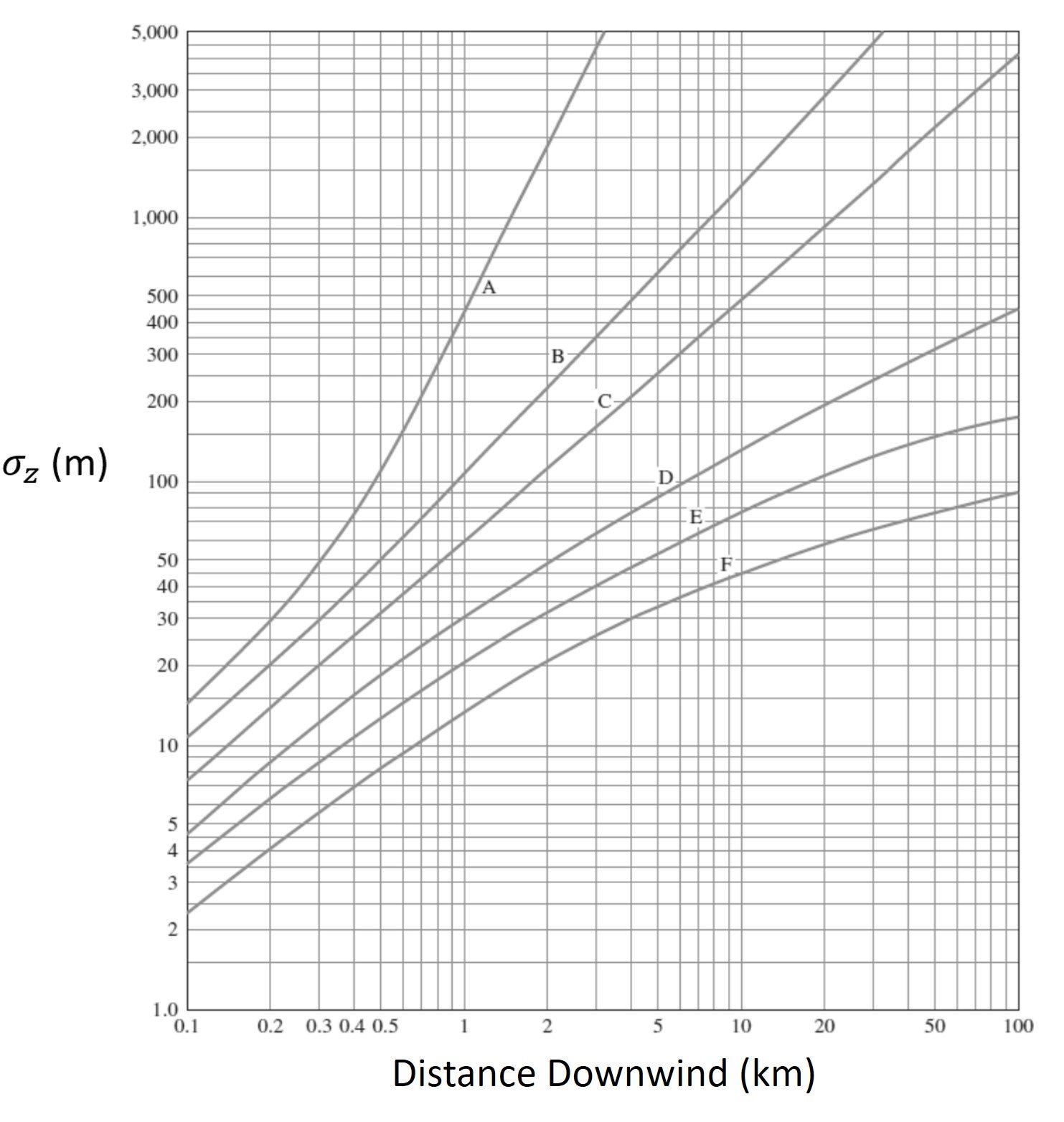
Once the atmospheric stability class has been determined and the desired downwind distance has been established, the dispersion coefficients can be read from Turner’s charts, Figures 2 and 3.

Figure 2. Dispersion coefficient $\displaystyle {{\sigma }_{y}}$ .

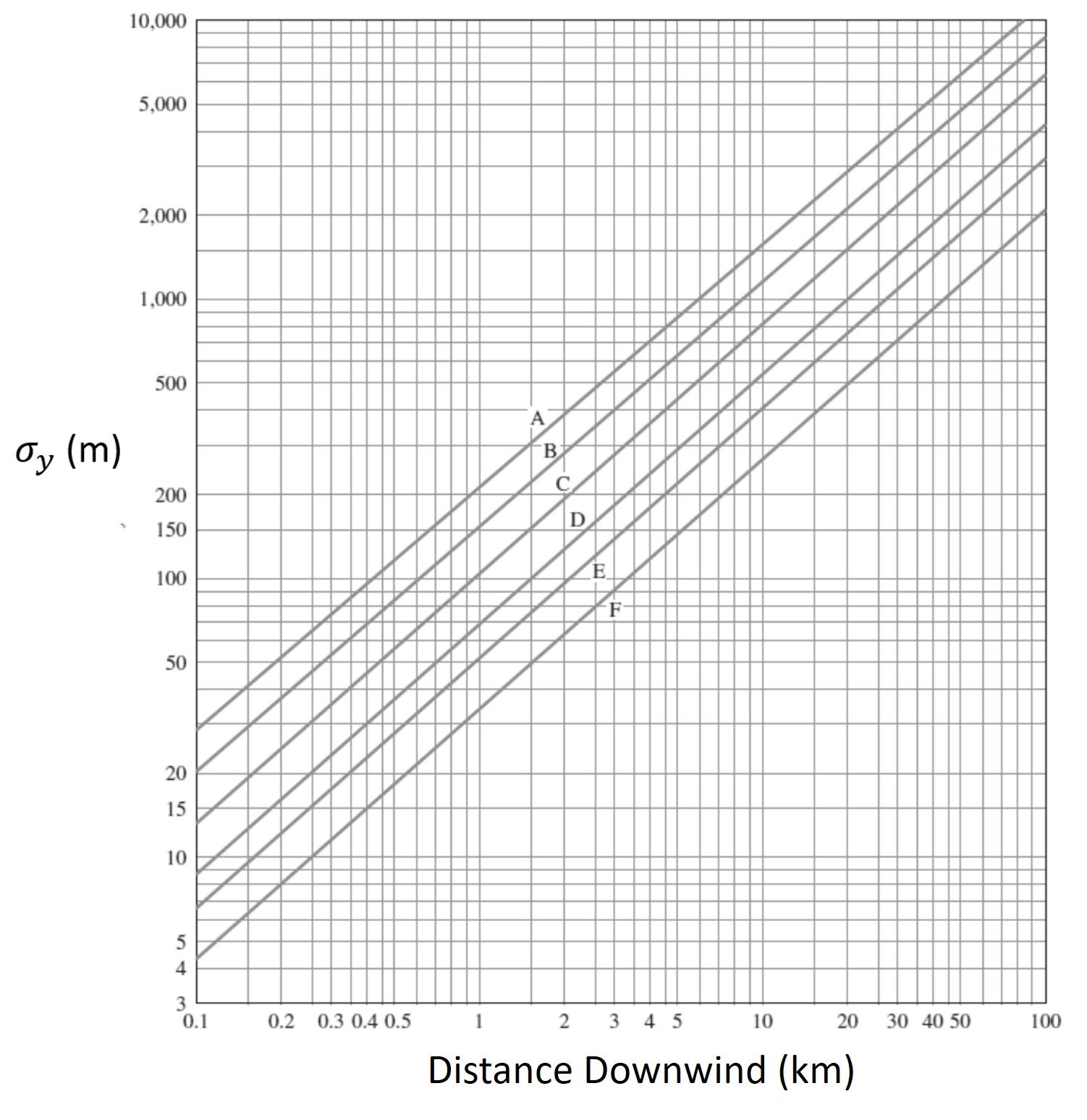
Figure 3. Dispersion coefficient $\displaystyle {{\sigma }_{z}}$ .

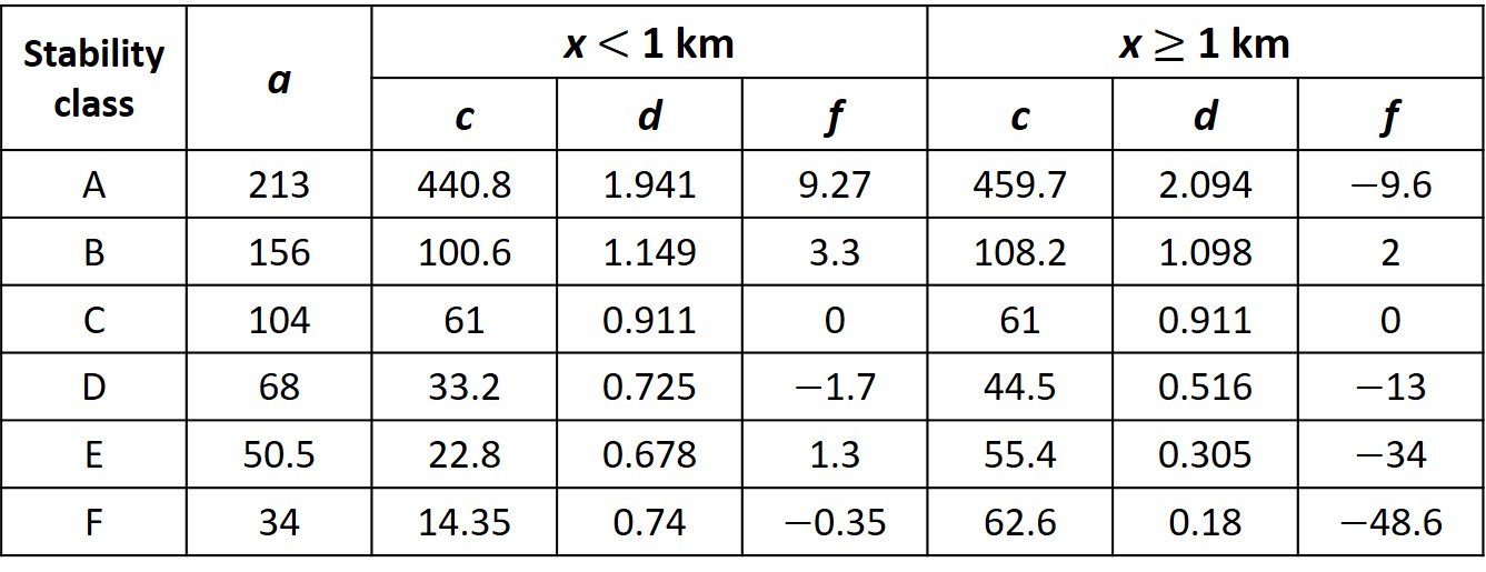
Use of the foregoing charts is tedious and not computer-friendly. In view of these limitations, two approximate formulas for $\displaystyle {{\sigma }_{y}}$ and $\displaystyle {{\sigma }_{z}}$ were developed, namely

$\displaystyle {{\sigma }_{y}}=a{{x}^{{0.894}}}$

$\displaystyle {{\sigma }_{z}}=c{{x}^{d}}+f$

where x is the downwind distance in kilometers and a, c, d and f are coefficients read from Table 2. Bear in mind that, while the value of x entered into these relations is in km, the outputs $\displaystyle {{\sigma }_{y}}$ and $\displaystyle {{\sigma }_{z}}$ are in meters.

Table 2. Coefficients for dispersion coefficient approximations

Use of the Gaussian plume equation also requires knowledge of wind speed. Wind speed varies with height, so that, unless the wind speed at the effective height of the plume is known, the wind speed must be corrected to account for the change in speed with elevation. For elevations up to a few hundred meters, a power law expression may be used to estimate the wind speed at heights other than that of the measurement,

$\displaystyle {{u}_{2}}={{u}_{1}}{{\left( {\frac{{{{z}_{2}}}}{{{{z}_{1}}}}} \right)}^{p}}$

where u₁ is wind speed at elevation z₁, u₂ is wind speed at elevation z₂, and p is an exponent. Values of p recommended by the US EPA for rural and urban environments are listed on Table 3.

Table 3. Exponent p for use with wind speed equation

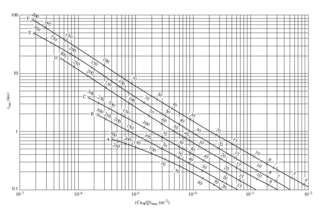
Turner also prepared a chart for computation of maximum pollutant concentration, namely

$\displaystyle {{C}_{{\max }}}=\frac{Q}{{{{u}_{H}}}}{{\left( {\frac{{C{{u}_{H}}}}{Q}} \right)}_{{\max }}}$

where factor (Cu_H/Q)_max is a normalized concentration that may be read from Figure 4, which provides this parameter as a function of atmospheric stability class and effective stack height.

Figure 4. To determine the downwind concentration peak, enter the graph at the appropriate stability classification and effective stack height (numbers on the graph, in meters) and then move across to find the distance to the peak, and down to find a parameter from which the peak concentration can be calculated. (Download full size picture here).

2. Solved Example

A stack emitting one mole of SO₂ per second has an effective stack height of 150 m. The windspeed is 2.5 m/s at 10 m, and it is a clear day in an urban environment with the sun 45^o above the horizon. Estimate the ground-level SO₂ concentration

A) Directly downwind at a distance of 1.5 km.

B) At a point located 1.5 km downwind and 200 m off the downwind axis.

C) At the point downwind where SO₂ is a maximum.

A) With reference to Table 1, the surface windspeed and insolation conditions in question correspond to atmospheric stability category B. From Table 2, we read coefficients a = 156, c = 108.2, d = 1.098, and f = 2. The dispersion coefficients are then

$\displaystyle {{\sigma }_{y}}=a{{x}^{{0.894}}}=156\times {{1.5}^{{0.894}}}=224\,\text{m}$

$\displaystyle {{\sigma }_{z}}=c{{x}^{d}}+f=108.2\times {{1.5}^{{1.098}}}+2=171\,\,\text{m}$

For stability class B and an urban setting, a wind speed exponent p = 0.15 is taken from Table 3. The wind speed at a stack height of 150 m follows as

$\displaystyle {{u}_{H}}={{u}_{1}}{{\left( {\frac{{{{z}_{2}}}}{{{{z}_{1}}}}} \right)}^{p}}=2.5\times {{\left( {\frac{{150}}{{10}}} \right)}^{{0.15}}}=3.75\,\,\text{m/s}$

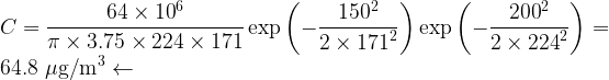
Noting that one mole of SO₂ corresponds to 64 $\displaystyle \times$ 10⁶ $\displaystyle \mu$ g, we can appeal to the Gaussian plume equation and determine the concentration at a distance of 1.5 km,

$\displaystyle C\left( {x,0} \right)=\frac{Q}{{\pi {{u}_{H}}{{\sigma }_{y}}{{\sigma }_{z}}}}\exp \left( {-\frac{{{{H}^{2}}}}{{2\sigma _{z}^{2}}}} \right)$

$\displaystyle C=\frac{{64\times {{{10}}^{6}}}}{{\pi \times 3.75\times 224\times 171}}\times \exp \left( {-\frac{{{{{150}}^{2}}}}{{2\times {{{171}}^{2}}}}} \right)=96.5\,\,\mu \text{g/}{{\text{m}}^{3}}\leftarrow$

B) Dispersion coefficients continue to be $\displaystyle {{\sigma }_{y}}$ = 224 m and $\displaystyle {{\sigma }_{z}}$ = 171 m, but the concentration is now

$\displaystyle C=\frac{{64\times {{{10}}^{6}}}}{{\pi \times 3.75\times 224\times 171}}\exp \left( {-\frac{{{{{150}}^{2}}}}{{2\times {{{171}}^{2}}}}} \right)\exp \left( {-\frac{{{{{200}}^{2}}}}{{2\times {{{224}}^{2}}}}} \right)=64.8\ \mu \text{g/}{{\text{m}}^{3}}\leftarrow$

C) Entering a stability class B and an effective stack height of 150 m into Figure 4, we see that the downwind concentration peak is achieved at x_max = 1 km and corresponds to a factor (Cu_H/Q)_max = 8 $\displaystyle \times$ 10^-6 m^-2. The concentration peak is then

$\displaystyle {{C}_{{\max }}}=\frac{Q}{{{{u}_{H}}}}{{\left( {\frac{{C{{u}_{H}}}}{Q}} \right)}_{{\max }}}=\frac{{\left( {64\times {{{10}}^{6}}} \right)}}{{3.75}}\times \left( {8\times {{{10}}^{{-6}}}} \right)=137\,\,\mu \text{g/}{{\text{m}}^{3}}\leftarrow$

3. Optimizing the Gaussian plume

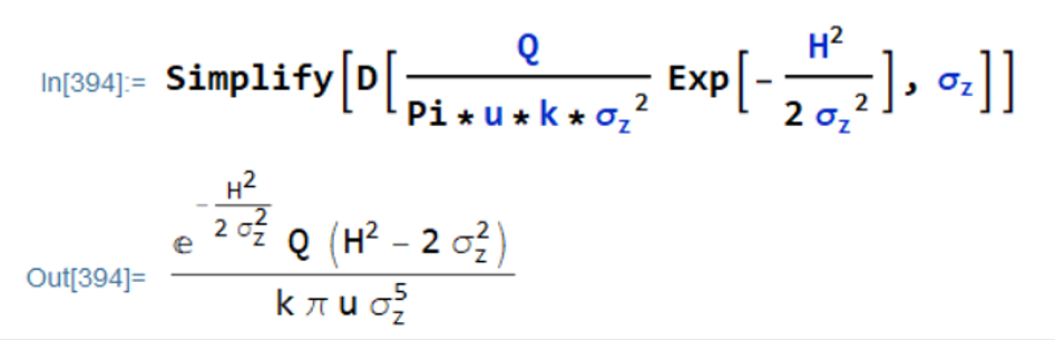
For stability class C, the ratio of dispersion coefficients $\displaystyle {{\sigma }_{y}}$ / $\displaystyle {{\sigma }_{z}}$ is essentially constant, that is, $\displaystyle {{\sigma }_{y}}$ = k $\displaystyle {{\sigma }_{z}}$ . In such a case, we can easily determine the distance downwind from a stack at which the maximum concentration occurs. To do so, we first differentiate the dispersion equation with respect to $\displaystyle {{\sigma }_{z}}$ , as in the Mathematica code

Then, we set the derivative to zero and solve for $\displaystyle {{\sigma }_{z}}$ ,

$\displaystyle {{H}^{2}}-2\sigma _{z}^{2}=0$

$\displaystyle \therefore {{\sigma }_{z}}=\frac{H}{{\sqrt{2}}}$

That is, the maximum concentration occurs at a point where dispersion coefficient $\displaystyle {{\sigma }_{z}}$ equals approximately 0.707H. Substituting this result in the plume equation, the maximum concentration C_max is obtained,

$\displaystyle {{C}_{{\max }}}=\frac{Q}{{\pi {{u}_{H}}{{\sigma }_{y}}{{\sigma }_{z}}}}\exp \left[ {-\frac{{{{H}^{2}}}}{{2\times {{{\left( {{H}/{{\sqrt{2}}}\;} \right)}}^{2}}}}} \right]=\frac{{0.117Q}}{{{{u}_{H}}{{\sigma }_{y}}{{\sigma }_{z}}}}$

Substituting $\displaystyle {{\sigma }_{y}}$ = k $\displaystyle {{\sigma }_{z}}$ and $\displaystyle {{\sigma }_{z}}$ = 0.707H brings to

$\displaystyle {{C}_{{\max }}}=\frac{{0.117Q}}{{{{u}_{H}}\times k{{\sigma }_{z}}\times 0.707H}}$

$\displaystyle \therefore {{C}_{{\max }}}=\frac{{0.117Q}}{{{{u}_{H}}\times k\times 0.707H\times 0.707H}}$

$\displaystyle \therefore {{C}_{{\max }}}=\frac{{0.234Q}}{{k{{u}_{H}}{{H}^{2}}}}$

Clearly, the maximum concentration is directly proportional to the emission rate of pollutants, and inversely proportional to wind velocity and effective stack height. Doubling the effective stack height would decrease the maximum concentration four-fold.

References

• MASTERS, G. and ELA, W. (2014). Introduction to Environmental Engineering and Science: Pearson New International Edition. 3rd edition. Upper Saddle River: Pearson.

• MIHELCIC, J. and ZIMMERMAN, J. (2014). Environmental Engineering. 2nd edition. Hoboken: John Wiley and Sons.

Air Pollution and the Gaussian Plume Model

Subscribe to our Mailing List!

Featured Posts

A Primer on NAND Flash Memories

Solidification Time and Chvorinov’s Rule

Step-Growth Polymerization, the Carothers Equation, and the Flory-Schulz Distribution

More Articles

Size Reduction, the Three Laws of Comminution, and the Bond Equation

Stomatal Conductance and Plant Transpiration

Fields of Study

More

© 2024 Montogue Quiz

Subscribe to
our Mailing List!

Subscribe to our Mailing List!

Subscribe to receive our latest materials in your inbox.

Homework Help

© 2024 Montogue Quiz

Subscribe to our Mailing List!