The Bruun Rule and Sea-Level Rise

1. Introduction

Global mean sea level rise (SLR) is the net result of geophysical and climatological processes. Hay et al. (2015) performed a statistical reanalysis of data from at the time and of their paper and placed the rate of increase of global mean sea-level at 1.20.2 millimeters per year for the period 1901 – 1990 and 3.00.7 mm/year for the period 1993 – 2010, implying that SLR has accelerated rapidly in recent years. According to recent projections by the Intergovernmental Panel on Climate Change (IPCC), global mean sea levels will rise between 0.43 m and 0.84 m by 2100 relative to the 1986 – 2005 period. Needless to say, communities in coastal areas, which house a substantial fraction of the global population, are particularly vulnerable to the potentially devastating effects that SLR is expected to cause, such as more severe coastal flooding regimes (Taherkhani et al., 2020). Therefore, managers in these areas must be equipped with some sort of relationship between shoreline recession and SLR; for over 50 years, the go-to model for this purpose has been the Bruun rule, whose advantages and shortcomings we discuss in the present article.

2. The Bruun rule

It seems prudent to take 100 years as the horizon for most planning exercises in the coastal zone and as a reasonable goal for the development of integrated coastal zone management. On this timescale, the approach or starting point of most research on the potential effect of sea-level rise globally, and at a local level, has long been the simple conceptual model proposed by Per Bruun in a1962 paper (Bruun, 1962). This publication, along with Schwartz (1967), sparked academic interest in problems of coastal recession and SLR, and offered stakeholders with a novel equation, now known as the Bruun rule, with which to base more thorough investigations.

The Bruun rule assumes that over the long term the “active” portion of a profile perpendicular to the shoreline maintains a constant form known as an equilibrium profile. Characteristics of the profile depend primarily on sand size (assumed constant) and secondarily on wave parameters. The active profile extends to a water depth known as “closure depth,” beyond which there is little sand motion and, according to Bruun, there is no movement of sand onto the active profile. The Bruun rule assumes that the active profile maintains its shape over the long term, but rises with sea-level rise. In order for the profile to move upward, there must be a source of sand, and the Bruun rule assumes that all of the sand is transported from the shoreline, and this loss of sand causes shoreline recession. Therefore, as shown in Figure 1, the shoreline change, R, due to sea-level rise S may be expressed as

Here, B is the height of the beach berm, L_* is the horizontal distance from the berm to the section of the closure depth, and h_* is the closure depth itself. Importantly, it is assumed that R  L_* and S  h_*. As noted by the Scientific Committee Working Group 89 (1991), the equation can be restated as

where tan  (B + h_*)/L_* is the average slope of the nearshore along the cross-shore width L_*. Since the slopes of many sandy profiles are in the range 0.01 – 0.02, the equation above predicts a landward movement of the shoreline ranging from 50S to 100S. Thus, a small increase in sea level is predicted to yield a substantial retreat of the shoreline. This predicted displacement is roughly the same as that which would occur from simple inundation of a linear profile, but what is different is the postulated sediment volume required to produce the upward shift of the equilibrium profile, and thus the nature of the processes controlling this change. As stated, it should be noted that the Bruun rule assumes that the height of the berm B is assumed to be much less than the depth of closure h_*. If B is large, as in the case of, say, a high dune, then the value of R predicted by the foregoing equation will be substantially reduced.

Figure 1. Illustration of shoreline regression.

The Bruun model is thus elegant in its simplicity. The matching of thickness of sediment deposited on the profile to the height of the sea-level rise means that the landward displacement of the shoreline is essentially a function of the profile slope and the vertical sea-level rise, as long as there is an abundant supply of sediment landward of the shoreline.

As stated, the Bruun rule is based on the notion of an equilibrium profile, which Bruun (1962) defined as “a statistical average profile which maintains its form apart from small fluctuations including seasonal fluctuations.” More recently, Larson and Wise (1998) stated, with reference to this concept, that “a beach of specific grain size, if exposed to constant forcing conditions, normally assumed to be short-period breaking waves, will develop a profile shape that displays no net change in time.” Of course, an equilibrium profile must be described with a simple mathematical expression; the simplest such expression is, as mentioned in Bruun (1954),

where h is water depth, x is distance offshore, and A is a shape factor. Dean (1977) verified this relationship using a profile dataset from Hayden et al. (1975) and corroborated the exponent value of 2/3 originally adopted by Bruun. Furthermore, Dean (1977) found that the shape factor A depends primarily on sediment characteristics and speculated that the monotonic profile form is consistent with uniform wave energy dissipation per unit volume of the water column within the surf zone. Later, Dean (1987) related A to sediment fall velocity by fitting available sediment grain size data to the equation

where w is the sediment fall velocity in cm/s. Inman et al. (1993) extended the model in question to the case represented by two segments of the same form as the Bruun power law but with different exponents and reference positions for the two segments; however, the Inman et al. representation is built upon seven parameters, making it difficult to apply and test against profiles in nature. As in so many areas of geomorphology, here we have a tradeoff between realism and simplicity.

3. Reviewing the assumptions and issues

As mentioned by Davidson-Arnott (2005), the three main assumptions upon which the Bruun rule is based are:

1. It applies to a two-dimensional profile normal to the shoreline so that all net sediment transfers are onshore-offshore and no consideration is given to inputs or outputs alongshore.
2. The profile is assumed to be an equilibrium profile entirely developed in sand, with the mean profile form reflecting the wave climate and the size of the sediment.
3. The material landward of the shoreline consists of easily erodible sand with characteristics similar to those in the nearshore.

3.1. Bidimensionality and no alongshore transport

The main assumption of the Bruun rule is that all sand transport occurs perpendicularly to the shoreline (i.e., cross-shore), which makes it a strictly two-dimensional model (though some workers have somewhat recklessly used it to tackle 3D problems as well). The model makes no allowance for sediment sinks/sources or alongshore gradients in net longshore transport. Accordingly, the Bruun rule does not account for any three-dimensional variability inherent to some natural coastlines, hindering its application in certain settings (see below). This important shortcoming of the Bruun rule was amply illustrated in a large-scale study of coastal recession along a 220 km stretch of the US East Coast, where almost 70% of the study area was excluded from the analysis to eliminate the influence of the many inlets and engineering structures located therein (Zhang et al., 2004).

3.2. The closure depth

The depth of closure delineates the nearshore (landward of the closure depth to the shoreline) from the offshore (seaward of the closure depth) and represents the threshold where bed sediments are no longer significantly transported by waves. In other words, it is assumed that all sediment erosion, transportation, and deposition occurs landward of the closure depth.

Predictably, the assumption that no significant amount of sediment escapes beyond an offshore seaward limit, that is, the closure depth, is questionable. Specification of closure depth is an important part of nourished beach design, since it basically determines the volume of sand required. However, in actuality the closure depth is a concept with little basis in reality. Significant amounts of sand transport on the continental shelf and the surf zone are well-documented, casting doubt on the idea that the two environments are separated by a zone of insignificant sediment movement.

The closure depth can be gleaned from sediment boundaries, profile slopes, or empirical formulations. Since detailed sediment grain size maps or bathymetric surveys are often not available, use of empirical correlations has been the prevailing source of closure depths for coastal modelling. Of course, these empirical correlations are themselves derived from uncertainty-ridden quantities (e.g., sediment size, wavebreaking depths, etc.) and, if used indiscriminately, may only worsen SLR estimates extracted from the Bruun rule.

3.3. The equilibrium profile

Convenient as the concept of equilibrium profile may be, the determination of a shoreline’s EP – assuming one exists at all – requires a dataset of regularly measured profiles that captures the envelope of profile changes associated with all water level and climate fluctuations. Technical and temporal constraints often prevent coastal modelers from obtaining such comprehensive data, so compromises in coastal modelling and design are adopted (Atkinson et al., 2018). For instance, in the absence of mean profiles, some investigators have adopted experimental designs with different proxies for SLR, such as rising lake levels (Hands, 1979), varying tidal ranges (Schwartz, 1967), and land subsidence (Mimura and Nobuoka, 1995; see also Fig. 2).

3.4. Sediment size

Dean (1987) noted that the Bruun rule assumed that sand on the active profile was of uniform size, which constitutes an unrealistic simplification because sand size generally varies along profiles, becoming finer in the offshore direction (as acknowledged by Bruun (1983)). Dean (1987) proposed an equilibrium profile concept that included sand-size variability along the active profile. In Dean’s framework, for a particular wave climate, a sand particle of a particular size will be in equilibrium when resting at a particular wave depth. Following SLR, the sand particle must move to shallower water to be back to the water depth at which it is in equilibrium. Therefore, in response to SLR, sand particles should move landward over time to re-achieve the equilibrium profile.

3.5. Applicability of the Bruun rule – summary

Preliminary assumptions aside, the Bruun rule may also be gravely affected by uncertainty in its inputs, namely the quantity of sea-level rise S and the slope of the active nearshore bed profile (= tan  = (B + h_*)/L_*). Ranasinghe and Stive (2009) note that the most recent sea level rise forecasts available at the time of their paper placed SLR by year 2100 ranging anywhere from 18 cm to 1.4 m; inputting these values of S into the Bruun rule, shoreline recession estimates could vary by almost 700%. The slope of the active nearshore bed profile is likewise associated with substantial uncertainty, especially with regard to the depth of closure h. As mentioned above, this parameter is often obtained via empirical correlations that may themselves yield widely disparate results. For example, Ranasinghe et al. (2012) applied four common depth of closure theories to a coastal study in Sydney, Australia, and found active profile slope estimates ranging from 0.0625 to 0.011. This uncertainty range in tan  alone would produce Bruun rule recession estimates that vary by about 500%. Combine the uncertainties associated with S and tan  and you’d end up with Bruun-rule estimates for SLR in Sydney, Australia, at year 2100 ranging from 3 m to 127 m – an uncertainty of 4000%.

Application of the Bruun rule is made more difficult by modelers’ limited ability to disentangle it from other factors that may induce shoreline change, especially in the many coasts wherein SLR is not dominated by shoreline recession. For example, Dean and Houston (2016) determined that inlets modified for navigation caused about 70% of shoreline recession on the 575 km-long Florida east coast. In a similar manner, SLR has produced only about 5 – 10% of the recession along The Netherlands’ shoreline, which is also endowed with several inlets (Stive et al., 1990). Zhang et al. (2004) could only use 24% of the shoreline they considered to evaluate the Bruun rule because the remainder of the shoreline was influenced by inlets and coastal engineering projects. Passeri et al. (2014) analyzed shoreline response to sea-level rise along the south Atlantic Bight and northern Gulf of Mexico, USA, and concluded that the Bruun rule could be used effectively to determine shoreline recession only in areas where there was little to no “background” erosion caused by other factors. Many shorelines also have been subjected to substantial beach nourishment, masking shoreline recession caused by sea-level rise.

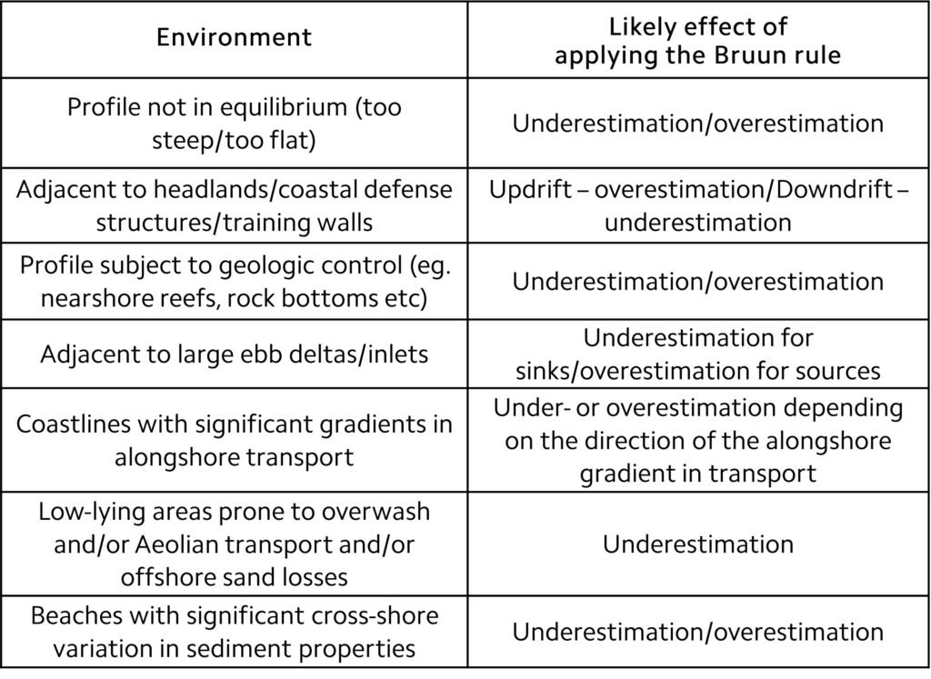
As summarized in Table 1, environments in which the Bruun rule is not immediately applicable include areas adjacent to headlands or engineering structures which control shoreline alignment, inlets/deltas which act as sediment sources or sinks, areas of significant gradients in alongshore sediment transport, low-lying overwash areas, and areas of significant sediment losses due to high Aeolian transport.

Table 1. Negative effects of applying the Bruun rule to estimate coastal recession due to SLR in various coastal environments. 

4. Testing the Bruun rule

With regard to regional Bruun rule applications, Rosen (1978) reported that a study in Chesapeake Bay considering 146 beach units yielded substantial errors in coastal recession when the rule was applied to specific sites, but when applied regionally (i.e., encompassing the entire bay) results were reasonably accurate. On the other hand, Dean (1990) compiled measured regional averaged erosion rates for 15 US states and found that almost all measurements fell outside the rule-of-thumb estimates of 50S – 100S (Ranasinghe, 2007).

In another noteworthy piece of research, Zhang et al. (2004) undertook a large-scale study of the US East Coast and contended that the poor agreement between Bruun rule predictions and actual data reported by Dean (1990) could be ascribed to the low quality of the measurements. Zhang’s group, using better quality data spanning 200 years for the US mid-Atlantic coast, found a surprisingly good agreement with the Bruun rule rule-of-thumb range (50S – 100S).

More recently, Atkinson et al. (2018), in a rare example of experimental validation, reported that in their experiments the Bruun rule predicted shoreline recession to within 25%, generally underpredicting the observations.

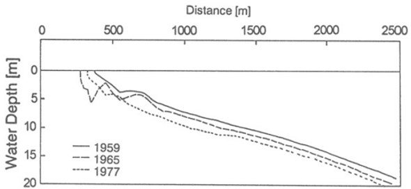
In an example of application from Asia, Mimura and Nobuoka (1995, Figure 2) reported on results from Niigata, Japan, over a period of 18 years during which groundwater withdrawal resulted in relative (subsidence coupled with limited sea-level rise) SLR rates up to 70 mm/year. 90 profile lines spaced at 100 m were surveyed 11 times during the 18 year period. Closure depths of 10 m and 17.5 m were considered. Plots show that the ratio of shoreline retreat to land subsidence is approximately 100. It was concluded that the “Bruun rule is verified to reproduce the past shoreline retreat very well.”

Figure 2. Three profiles presented by Mimura and Nobuoka (1995) in their evaluation of the Bruun rule for the Niigata, Japan area which experienced high subsidence over the study period. Note the parallel profiles for depths greater than 10 m supporting the choice of 10 m for depth of closure.

Some workers have attempted to modify the Bruun rule and hopefully make it more realistic. For instance, Davidson-Arnott (2005), starting from essentially the same assumptions that underpin the Bruun rule, conceived a model that includes beach-dune interaction and landward sediment transfer by Aeolian processes (Figure 3). Ranasinghe et al. (2012) incorporated SLR-driven landward movement of coastlines, a phenomenon that they called the ‘Bruun effect,’ into a robust model for climactic change-induced SLR in barrier estuaries. Rosati et al. (2013) proposed a modified version of the Bruun rule that considers the full range of parsing cross-shore transport, from completely seaward to completely landward, depending on the prevailing storm conditions and whether there is a surplus or deficit of sand in the profile with respect to the equilibrium beach profile. More recently, Dean and Houston (2016) proposed a modified Bruun rule with a host of additional terms, all the while accounting for aspects such as sediment sources/sinks and alongshore transport gradients.

Figure 3. Schematic illustration of the Davidson-Arnott (2005) model for response to sea-level rise showing erosion and landward migration of the nearshore profile and transgression of the beach and foredune.

5. Conclusion

Outright abandonment of the Bruun rule has been suggested by Cooper and Pilkey (2004). In spite of its many shortcomings, the rule remains an essential component of numerous studies and models of coastal response (e.g., Hanson, 1989; Dean, 1991; Ranasinghe et al., 2012; Vousdoukas et al., 2020). Further, as indicated by some of the studies quoted above, the Bruun rule has been successfully evoked in models of barrier translation (Dean and Maurmeyer, 1983), landward transport (Rosati et al., 2013), and the dune-sediment budget (Davidson-Arnott, 2005), to name a few.

Following a comprehensive review of attempts to test the rule, Scientific Committee Working Group 89 (1991), working on behalf of the Scientific Committee on Oceanic Research, concluded that while conceptually correct, recession rates predicted by the rule can differ from measured rates by large factors. Accordingly, SCOR recommended that the rule be used only for order-of-magnitude estimates of potential recession. At best, any predictions obtained via the Bruun rule should be considered as broadly indicative estimates that are not suitable for direct use in coastal planning and management.

References

Download references list here.