
In this article, I provide a quick introduction to some of the most important parameters and results of physical geodesy. Section 1 is a derivation of Clairaut’s theorem, an equation that bridges the geometric and gravitational facets of geodetic science. Section 2 introduces J2, a coefficient, known by names such as “dynamic oblateness” (Stacey and Davis, 2008) and “dynamic form factor” (Buforn et al., 2012), that has grown in importance enormously since the advent of artificial satellites and thus deserves a few paragraphs of its own. The material of sections 1 and 2 is then applied in two example problems. The article closes with a section on Clairaut’s differential equation and how it can be related to the Earth’s shape, its internal density distribution, and beyond.
1. Flattening and Clairaut’s theorem
In the following developments, (u,

Normal gravity, often denoted by 

where

is the line element for elliptical coordinate u, i.e. the change du that yields the distance change sudu, h is the geodetic height, which is along the normal to the reference ellipsoid, and E is the linear eccentricity. Normal gravity on the ellipsoid (
![\displaystyle {{\gamma }_{0}}=\frac{{GM}}{{{{a}^{2}}\Psi }}\left[ {1+m{e}'\frac{{{q}'\left( b \right)}}{{q\left( b \right)}}\left( {\frac{{{{{\sin }}^{2}}\beta }}{2}-\frac{1}{6}} \right)-m{{{\cos }}^{2}}\beta } \right]\,\,\,(2)](https://s0.wp.com/latex.php?latex=%5Cdisplaystyle+%7B%7B%5Cgamma+%7D_%7B0%7D%7D%3D%5Cfrac%7B%7BGM%7D%7D%7B%7B%7B%7Ba%7D%5E%7B2%7D%7D%5CPsi+%7D%7D%5Cleft%5B+%7B1%2Bm%7Be%7D%27%5Cfrac%7B%7B%7Bq%7D%27%5Cleft%28+b+%5Cright%29%7D%7D%7B%7Bq%5Cleft%28+b+%5Cright%29%7D%7D%5Cleft%28+%7B%5Cfrac%7B%7B%7B%7B%7B%5Csin+%7D%7D%5E%7B2%7D%7D%5Cbeta+%7D%7D%7B2%7D-%5Cfrac%7B1%7D%7B6%7D%7D+%5Cright%29-m%7B%7B%7B%5Ccos+%7D%7D%5E%7B2%7D%7D%5Cbeta+%7D+%5Cright%5D%5C%2C%5C%2C%5C%2C%282%29&bg=ffffff&fg=000&s=1&c=20201002)
Here, G is the gravitational constant, M is the mass of the Earth, a is the equatorial semiaxis, b is the polar semiaxis, 
where 
![\displaystyle {q}'\left( u \right)=-\frac{{{{u}^{2}}+{{E}^{2}}}}{E}\frac{{dq}}{{du}}=3\left( {1+\frac{{{{u}^{2}}}}{{{{E}^{2}}}}} \right)\left[ {1-\frac{u}{E}\arctan \left( {\frac{E}{u}} \right)} \right]-1\,\,\,(4)](https://s0.wp.com/latex.php?latex=%5Cdisplaystyle+%7Bq%7D%27%5Cleft%28+u+%5Cright%29%3D-%5Cfrac%7B%7B%7B%7Bu%7D%5E%7B2%7D%7D%2B%7B%7BE%7D%5E%7B2%7D%7D%7D%7D%7BE%7D%5Cfrac%7B%7Bdq%7D%7D%7B%7Bdu%7D%7D%3D3%5Cleft%28+%7B1%2B%5Cfrac%7B%7B%7B%7Bu%7D%5E%7B2%7D%7D%7D%7D%7B%7B%7B%7BE%7D%5E%7B2%7D%7D%7D%7D%7D+%5Cright%29%5Cleft%5B+%7B1-%5Cfrac%7Bu%7D%7BE%7D%5Carctan+%5Cleft%28+%7B%5Cfrac%7BE%7D%7Bu%7D%7D+%5Cright%29%7D+%5Cright%5D-1%5C%2C%5C%2C%5C%2C%284%29&bg=ffffff&fg=000&s=0&c=20201002)
where q is defined as
![\displaystyle iq\left( u \right)=\frac{i}{2}\left[ {\left( {1+\frac{{3{{u}^{2}}}}{{{{E}^{2}}}}} \right)\arctan \left( {\frac{E}{u}} \right)-3\frac{u}{E}} \right]\,\,\,(5)](https://s0.wp.com/latex.php?latex=%5Cdisplaystyle+iq%5Cleft%28+u+%5Cright%29%3D%5Cfrac%7Bi%7D%7B2%7D%5Cleft%5B+%7B%5Cleft%28+%7B1%2B%5Cfrac%7B%7B3%7B%7Bu%7D%5E%7B2%7D%7D%7D%7D%7B%7B%7B%7BE%7D%5E%7B2%7D%7D%7D%7D%7D+%5Cright%29%5Carctan+%5Cleft%28+%7B%5Cfrac%7BE%7D%7Bu%7D%7D+%5Cright%29-3%5Cfrac%7Bu%7D%7BE%7D%7D+%5Cright%5D%5C%2C%5C%2C%5C%2C%285%29&bg=ffffff&fg=000&s=1&c=20201002)
Using the formula above, normal gravities at the equator (
![\displaystyle {{\gamma }_{a}}=\frac{{GM}}{{ab}}\left[ {1-m-\frac{{m{e}'}}{6}\frac{{{q}'\left( b \right)}}{{q\left( b \right)}}} \right]\,\,\,(6)](https://s0.wp.com/latex.php?latex=%5Cdisplaystyle+%7B%7B%5Cgamma+%7D_%7Ba%7D%7D%3D%5Cfrac%7B%7BGM%7D%7D%7B%7Bab%7D%7D%5Cleft%5B+%7B1-m-%5Cfrac%7B%7Bm%7Be%7D%27%7D%7D%7B6%7D%5Cfrac%7B%7B%7Bq%7D%27%5Cleft%28+b+%5Cright%29%7D%7D%7B%7Bq%5Cleft%28+b+%5Cright%29%7D%7D%7D+%5Cright%5D%5C%2C%5C%2C%5C%2C%286%29&bg=ffffff&fg=000&s=1&c=20201002)
![\displaystyle {{\gamma }_{b}}=\frac{{GM}}{{{{a}^{2}}}}\left[ {1+\frac{{m{e}'}}{3}\frac{{{q}'\left( b \right)}}{{q\left( b \right)}}} \right]\,\,\,(7)](https://s0.wp.com/latex.php?latex=%5Cdisplaystyle+%7B%7B%5Cgamma+%7D_%7Bb%7D%7D%3D%5Cfrac%7B%7BGM%7D%7D%7B%7B%7B%7Ba%7D%5E%7B2%7D%7D%7D%7D%5Cleft%5B+%7B1%2B%5Cfrac%7B%7Bm%7Be%7D%27%7D%7D%7B3%7D%5Cfrac%7B%7B%7Bq%7D%27%5Cleft%28+b+%5Cright%29%7D%7D%7B%7Bq%5Cleft%28+b+%5Cright%29%7D%7D%7D+%5Cright%5D%5C%2C%5C%2C%5C%2C%287%29&bg=ffffff&fg=000&s=1&c=20201002)
Normal gravity at the equator, 


which I invite the reader to verify by substituting, in its left member, eqs. 6 and 7, along with b = a
In the 1920s, Somagliana (quoted in Sjöberg and Bagherbandi, 2017) developed an elegant closed formula for normal gravity on the ellipsoid,
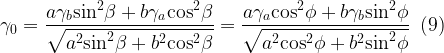
where, in addition to familiar variables, we have the geocentric latitude 
Hofmann-Wellenhof and Moritz (2005) develop an approximation to the gravity field that is linear relatively to the flattening f. The mathematical basis of the approximation is simple; first, note that the radius vector r of an ellipsoid can be approximated as

where a is equatorial radius, f is (terrestrial, geometric) flattening, and

where


Substituting f and f* into equation 8, we get

where

Equation 12 is Clairaut’s theorem in its original form. As pointed out by Hofmann-Wellenhof and Moritz (2005), this is one of the most striking formulas in physical geodesy, as it enables one to determine the geometrical flattening f from f* and m, which are purely dynamical quantities obtained by gravity measurements; that is, the flattening of the Earth can be determined from gravity measurements.
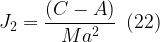
2. The dynamic oblateness or dynamic form factor J2
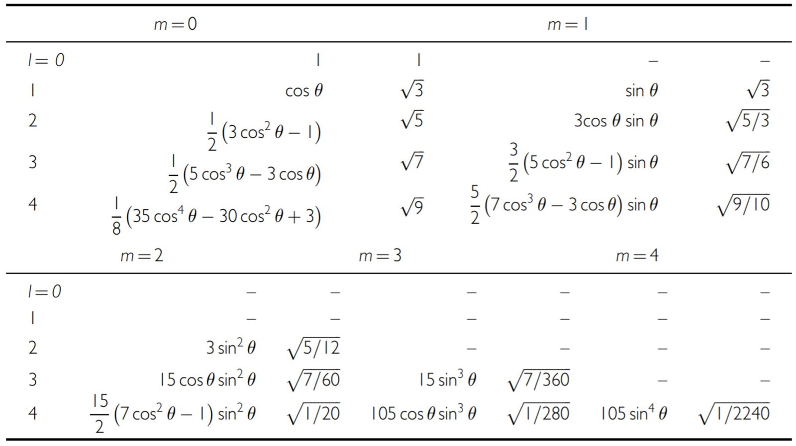
The gravitational potential due to the Earth at points external to it satisfies Laplace’s equation. Solutions for this equation in spherical polar coordinates, that are appropriate for the Earth’s sphericity, can be found in Stacey and Davis (2008). In cases of axial symmetry, the potential variation on a spherical surface can be treated as a sum of Legendre polynomials, Pl(cos 


Here, a is the equatorial radius, G is the gravitational constant, and coefficients J0, J1, J2, … represent the distribution of mass. By writing the equation in this form, we make these coefficients essentially dimensionless.
Since P0 = 1, we must have J0 = 1, because at great distances the first term becomes dominant and this gives the potential due to a point mass (or spherically symmetrical mass). By choosing the coordinate origin to be the center of mass, we must put J1 = 0, because P1 = cos

Stacey and Davis (2008) note that this is the potential at a stationary point, not rotating with the Earth, and that a rotating potential term must be added for points rotating with the Earth. Equation 15 gives the potential seen by satellites, including the Moon.
Table 1. Legendre polynomials 


It is useful to express the dynamic form factor J2 in terms of the principal moments of inertia of the Earth. To do so, we can appeal to MacCullagh’s formula, which gives the planet’s potential as

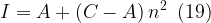
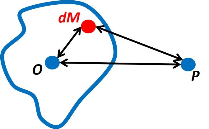
Here, A, B, and C are the moments of inertia of the Earth with respect to the x-, y-, and z-axes, respectively, and I is the moment of inertia of M about the axis OP (Figure 1). To identify equation 16 more closely with eq. 15, we write l in terms of A, B, C and the cosines l, m, n of the angles made by OP with the x, y, z axes:

where

This is simplified by introducing rotational symmetry about z, so that B = A and, substituting for B in 17 and also for l2 + m2 by equation 18, we have
and MacCullagh’s equation can be restated as

Since n = cos

which coincides with equation 15 inasmuch as
From satellite orbits,

In the first-order approximation, J2 can be related to flattening and the m coefficient by the simple expression

Figure 1. Points in the derivation of MacCullogh’s formula. dM is an infinitesimal mass element; O is the center of mass; P is an arbitrary point of interest. Moment of inertia I is determined with respect to axis OP. See Stacey and Davis (2008) for details.
Example 1
Point P is located at latitude 60oS on the terrestrial ellipsoid and has a distance to its center equal to 6360.44 km. Earth’s mass is 5.9761
Noting that the polar-to-equatorial ratio equals 0.9966, determining the terrestrial flattening is straightforward,


To find the dynamic oblateness J2 from equation 23, we first need the m coefficient. This in turn calls for the equatorial radius a, which is given by

so that, using the approximation a2b 


Substituting f and m into eq. 23 brings to


To find the normal gravity at point P, we first establish the gravity flattening via Clairaut’s theorem,

so that
![\displaystyle {{\gamma }_{P}}={{\gamma }_{a}}\left( {1+f*{{{\sin }}^{2}}\phi } \right)=978.032\times \left[ {1+\left( {5.195\times {{{10}}^{{-3}}}} \right)\times {{{\sin }}^{2}}60{}^\text{o}} \right]](https://s0.wp.com/latex.php?latex=%5Cdisplaystyle+%7B%7B%5Cgamma+%7D_%7BP%7D%7D%3D%7B%7B%5Cgamma+%7D_%7Ba%7D%7D%5Cleft%28+%7B1%2Bf%2A%7B%7B%7B%5Csin+%7D%7D%5E%7B2%7D%7D%5Cphi+%7D+%5Cright%29%3D978.032%5Ctimes+%5Cleft%5B+%7B1%2B%5Cleft%28+%7B5.195%5Ctimes+%7B%7B%7B10%7D%7D%5E%7B%7B-3%7D%7D%7D%7D+%5Cright%29%5Ctimes+%7B%7B%7B%5Csin+%7D%7D%5E%7B2%7D%7D60%7B%7D%5E%5Ctext%7Bo%7D%7D+%5Cright%5D&bg=ffffff&fg=000&s=0&c=20201002)
Example 2 shows that Clairaut’s classical geodesy can also be applied with reasonable accuracy to other astronomical bodies, such as the Moon.
Example 2
Assuming that the Moon is an ellipsoid of equatorial radius 1738 km and polar radius 1737 km, with dynamic oblateness J2 = 5.75374
First, we calculate the (lunar) flattening fM,

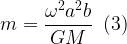
Then, we proceed to determine coefficient m,


From the definition of m, we can determine the period of rotation T,

![\displaystyle \therefore T={{\left[ {\frac{{4{{\pi }^{2}}\times {{{\left( {1738\times {{{10}}^{3}}} \right)}}^{3}}}}{{\left( {7.589\times {{{10}}^{{-6}}}} \right)\times \left( {6.674\times {{{10}}^{{-11}}}} \right)\times \left( {7.3483\times {{{10}}^{{22}}}} \right)}}} \right]}^{{{1}/{2}\;}}}=2.3598\times {{10}^{6}}\,\text{s}](https://s0.wp.com/latex.php?latex=%5Cdisplaystyle+%5Ctherefore+T%3D%7B%7B%5Cleft%5B+%7B%5Cfrac%7B%7B4%7B%7B%5Cpi+%7D%5E%7B2%7D%7D%5Ctimes+%7B%7B%7B%5Cleft%28+%7B1738%5Ctimes+%7B%7B%7B10%7D%7D%5E%7B3%7D%7D%7D+%5Cright%29%7D%7D%5E%7B3%7D%7D%7D%7D%7B%7B%5Cleft%28+%7B7.589%5Ctimes+%7B%7B%7B10%7D%7D%5E%7B%7B-6%7D%7D%7D%7D+%5Cright%29%5Ctimes+%5Cleft%28+%7B6.674%5Ctimes+%7B%7B%7B10%7D%7D%5E%7B%7B-11%7D%7D%7D%7D+%5Cright%29%5Ctimes+%5Cleft%28+%7B7.3483%5Ctimes+%7B%7B%7B10%7D%7D%5E%7B%7B22%7D%7D%7D%7D+%5Cright%29%7D%7D%7D+%5Cright%5D%7D%5E%7B%7B%7B1%7D%2F%7B2%7D%5C%3B%7D%7D%7D%3D2.3598%5Ctimes+%7B%7B10%7D%5E%7B6%7D%7D%5C%2C%5Ctext%7Bs%7D&bg=ffffff&fg=000&s=0&c=20201002)

3. Wahr’s (1996) rotating fluid sphere
Class notes by Wahr (1996) provide an interesting insight into the P2 term that pops up over and over in classical geodetic models. Why does rotation causes such a term, he asks, and why are the results for J2, f, and B2 (the latter of which we do not address here) equal to the numbers that they are equal to? What do these numerical values tell us about the Earth?
It turns out, Wahr answers, that the numerical results are consistent with the assumption that the Earth responds to the centrifugal force of rotation as though it were a fluid. To understand this result, Wahr proposes a simple model of a spherically symmetric fluid sphere (density = constant on spherical surfaces). We spin the fluid about the z-axis with an angular velocity
![\displaystyle r={{r}_{0}}\left[ {1-\frac{2}{3}\sum\limits_{{l=0}}^{\infty }{{{{\varepsilon }_{l}}\left( {{{r}_{0}}} \right){{P}_{l}}\left( {\cos \theta } \right)}}} \right]\,\,\,(24)](https://s0.wp.com/latex.php?latex=%5Cdisplaystyle+r%3D%7B%7Br%7D_%7B0%7D%7D%5Cleft%5B+%7B1-%5Cfrac%7B2%7D%7B3%7D%5Csum%5Climits_%7B%7Bl%3D0%7D%7D%5E%7B%5Cinfty+%7D%7B%7B%7B%7B%5Cvarepsilon+%7D_%7Bl%7D%7D%5Cleft%28+%7B%7B%7Br%7D_%7B0%7D%7D%7D+%5Cright%29%7B%7BP%7D_%7Bl%7D%7D%5Cleft%28+%7B%5Ccos+%5Ctheta+%7D+%5Cright%29%7D%7D%7D+%5Cright%5D%5C%2C%5C%2C%5C%2C%2824%29&bg=ffffff&fg=000&s=1&c=20201002)
where 


Accordingly, Wahr models constant density/VT (gravitational potential) surfaces with a shape described by
![\displaystyle r={{r}_{0}}\left[ {1-\frac{2}{3}\varepsilon \left( {{{r}_{0}}} \right){{P}_{2}}\left( {\cos \theta } \right)} \right]\,\,\,(25)](https://s0.wp.com/latex.php?latex=%5Cdisplaystyle+r%3D%7B%7Br%7D_%7B0%7D%7D%5Cleft%5B+%7B1-%5Cfrac%7B2%7D%7B3%7D%5Cvarepsilon+%5Cleft%28+%7B%7B%7Br%7D_%7B0%7D%7D%7D+%5Cright%29%7B%7BP%7D_%7B2%7D%7D%5Cleft%28+%7B%5Ccos+%5Ctheta+%7D+%5Cright%29%7D+%5Cright%5D%5C%2C%5C%2C%5C%2C%2825%29&bg=ffffff&fg=000&s=1&c=20201002)
where 

Finding the gravitational potential is much harder. Wahr presses on with a lengthy exercise on shell-shaped infinitesimal contributions to gravitational potential to find the overall gravitational potential V. To find V (r,
We must then determine
![\displaystyle -\frac{8}{5}\pi G\left\{ {\frac{1}{{r_{1}^{3}}}\int_{0}^{{{{r}_{1}}}}{{\rho \left( {{{r}_{0}}} \right)r_{0}^{4}}}\left[ {5\varepsilon \left( {{{r}_{0}}} \right)+{{r}_{0}}{{\partial }_{{r0}}}\varepsilon \left( {{{r}_{0}}} \right)} \right]d{{r}_{0}}+r_{1}^{2}\int_{{{{r}_{1}}}}^{a}{{\rho \left( {{{r}_{0}}} \right){{\partial }_{{r0}}}\varepsilon \left( {{{r}_{0}}} \right)d{{r}_{0}}}}-5\frac{{\varepsilon \left( {{{r}_{1}}} \right)}}{{{{r}_{1}}}}\int_{0}^{{{{r}_{1}}}}{{\rho \left( {{{r}_{0}}} \right)r_{0}^{2}d{{r}_{0}}}}} \right\}={{\omega }^{2}}r_{1}^{2}\,\,\,(26)](https://s0.wp.com/latex.php?latex=%5Cdisplaystyle+-%5Cfrac%7B8%7D%7B5%7D%5Cpi+G%5Cleft%5C%7B+%7B%5Cfrac%7B1%7D%7B%7Br_%7B1%7D%5E%7B3%7D%7D%7D%5Cint_%7B0%7D%5E%7B%7B%7B%7Br%7D_%7B1%7D%7D%7D%7D%7B%7B%5Crho+%5Cleft%28+%7B%7B%7Br%7D_%7B0%7D%7D%7D+%5Cright%29r_%7B0%7D%5E%7B4%7D%7D%7D%5Cleft%5B+%7B5%5Cvarepsilon+%5Cleft%28+%7B%7B%7Br%7D_%7B0%7D%7D%7D+%5Cright%29%2B%7B%7Br%7D_%7B0%7D%7D%7B%7B%5Cpartial+%7D_%7B%7Br0%7D%7D%7D%5Cvarepsilon+%5Cleft%28+%7B%7B%7Br%7D_%7B0%7D%7D%7D+%5Cright%29%7D+%5Cright%5Dd%7B%7Br%7D_%7B0%7D%7D%2Br_%7B1%7D%5E%7B2%7D%5Cint_%7B%7B%7B%7Br%7D_%7B1%7D%7D%7D%7D%5E%7Ba%7D%7B%7B%5Crho+%5Cleft%28+%7B%7B%7Br%7D_%7B0%7D%7D%7D+%5Cright%29%7B%7B%5Cpartial+%7D_%7B%7Br0%7D%7D%7D%5Cvarepsilon+%5Cleft%28+%7B%7B%7Br%7D_%7B0%7D%7D%7D+%5Cright%29d%7B%7Br%7D_%7B0%7D%7D%7D%7D-5%5Cfrac%7B%7B%5Cvarepsilon+%5Cleft%28+%7B%7B%7Br%7D_%7B1%7D%7D%7D+%5Cright%29%7D%7D%7B%7B%7B%7Br%7D_%7B1%7D%7D%7D%7D%5Cint_%7B0%7D%5E%7B%7B%7B%7Br%7D_%7B1%7D%7D%7D%7D%7B%7B%5Crho+%5Cleft%28+%7B%7B%7Br%7D_%7B0%7D%7D%7D+%5Cright%29r_%7B0%7D%5E%7B2%7Dd%7B%7Br%7D_%7B0%7D%7D%7D%7D%7D+%5Cright%5C%7D%3D%7B%7B%5Comega+%7D%5E%7B2%7D%7Dr_%7B1%7D%5E%7B2%7D%5C%2C%5C%2C%5C%2C%2826%29&bg=ffffff&fg=000&s=0&c=20201002)
using r1 instead of r0 to distinguish between the field (r1) point and the mass (r0) point. Equation 26 is an integral equation in 


In condensed notation,
![\displaystyle \bar{\rho }\left( r \right)\left[ {\partial _{r}^{2}\varepsilon \left( r \right)-\frac{6}{{{{r}^{2}}}}\varepsilon \left( r \right)} \right]+\frac{{6\rho \left( r \right)}}{r}\left[ {{{\partial }_{r}}\varepsilon \left( r \right)+\frac{{\varepsilon \left( r \right)}}{r}} \right]=0\,\,\,(28)](https://s0.wp.com/latex.php?latex=%5Cdisplaystyle+%5Cbar%7B%5Crho+%7D%5Cleft%28+r+%5Cright%29%5Cleft%5B+%7B%5Cpartial+_%7Br%7D%5E%7B2%7D%5Cvarepsilon+%5Cleft%28+r+%5Cright%29-%5Cfrac%7B6%7D%7B%7B%7B%7Br%7D%5E%7B2%7D%7D%7D%7D%5Cvarepsilon+%5Cleft%28+r+%5Cright%29%7D+%5Cright%5D%2B%5Cfrac%7B%7B6%5Crho+%5Cleft%28+r+%5Cright%29%7D%7D%7Br%7D%5Cleft%5B+%7B%7B%7B%5Cpartial+%7D_%7Br%7D%7D%5Cvarepsilon+%5Cleft%28+r+%5Cright%29%2B%5Cfrac%7B%7B%5Cvarepsilon+%5Cleft%28+r+%5Cright%29%7D%7D%7Br%7D%7D+%5Cright%5D%3D0%5C%2C%5C%2C%5C%2C%2828%29&bg=ffffff&fg=000&s=1&c=20201002)
where

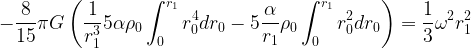
As an example, Wahr assumes 

In this case, Clairaut’s equation reduces to

Wahr proposes a solution of the form 


so n = 0 or n = –5. It follows that the general solution has the form

It remains to determine coefficients 


The real density inside the Earth is not constant, but increases with depth. It turns out that Clairaut’s equation implies that

![\displaystyle r\left( {\theta =90{}^\text{o}} \right)-r\left( {\theta =0{}^\text{o}} \right)=-\frac{2}{3}\varepsilon {{r}_{0}}\left[ {{{P}_{2}}\left( {90{}^\text{o}} \right)-{{P}_{2}}\left( {0{}^\text{o}} \right)} \right]](https://s0.wp.com/latex.php?latex=%5Cdisplaystyle+r%5Cleft%28+%7B%5Ctheta+%3D90%7B%7D%5E%5Ctext%7Bo%7D%7D+%5Cright%29-r%5Cleft%28+%7B%5Ctheta+%3D0%7B%7D%5E%5Ctext%7Bo%7D%7D+%5Cright%29%3D-%5Cfrac%7B2%7D%7B3%7D%5Cvarepsilon+%7B%7Br%7D_%7B0%7D%7D%5Cleft%5B+%7B%7B%7BP%7D_%7B2%7D%7D%5Cleft%28+%7B90%7B%7D%5E%5Ctext%7Bo%7D%7D+%5Cright%29-%7B%7BP%7D_%7B2%7D%7D%5Cleft%28+%7B0%7B%7D%5E%5Ctext%7Bo%7D%7D+%5Cright%29%7D+%5Cright%5D&bg=ffffff&fg=000&s=1&c=20201002)
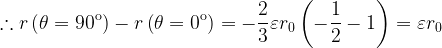
So,
Finally, Wahr (1996) notes that, using the best seismic results for the density function
One possible reason for the poor prediction of flattening/dynamical ellipticity in the Clairaut model is that the mantle is a very viscous fluid and, in view of its exceptionally large viscosity, it takes a reasonably long time for the mantle to reach equilibrium. The relevance of this is that the Earth’s rotation is decreasing approximately linearly with time, and so the centrifugal force is decreasing. If the viscosity is high enough that the mantle response time is longer than the time it takes for the centrifugal force to decrease significantly, then the present shape of the Earth might be reflecting the older, faster rotation. This would lead to ellipticities larger than those predicted from Clairaut’s equation. Most geophysicists do not subscribe to this explanation, however. Indeed, estimates of mantle viscosity from postglacial rebound suggest the viscosity is not large enough to support this hypothesis.
Wahr concludes that the most likely explanation is that the Earth is approximately fluid over long time periods, but that there are other factors besides rotation that cause lateral variations in density. That is certainly the case: thermal anomalies must exist within the Earth if there is to be ongoing mantle convection. Those thermal anomalies must be associated with density anomalies (it is buoyancy forces caused by the density anomalies that directly drive the convection). So, presumably the discrepancy from Clairaut’s equation is due to the spherico-harmonic 
References
• BUFORN, E., PRO, C. and UDÍAS, A. (2012). Solved Problems in Geophysics. Cambridge: Cambridge University Press.
• HEISKANEN, W. and MORITZ, H. (1967). Physical Geodesy. New York: W.H. Freeman.
• HOFMANN-WELLENHOF, B. and MORITZ, H. (2005). Physical Geodesy. Vienna: Springer Wien.
• SJÖBERG, L. and BAGHERBANDI, B. (2017). Gravity Inversion and Gravitation. Berlin/Heidelberg: Springer.
• STACEY, M. and DAVIS, F. (2008). Physics of the Earth. 4th edition. Cambridge: Cambridge University Press.
• WAHR, J. (1996). Geodesy and Gravity: Class Notes. Boulder: University of Colorado.