Glacier Profiles: The Parabolic, Vialov, and Bueler Models

In this blog post, we discuss how some basic thermomechanical characteristics of ice can be used to predict the geometry of a glacier or ice sheet. Three models are introduced; before discussing them, however, the reader should be introduced to Glen’s flow law, the most widely used constitutive law for creep of mineral ice. If you’re already acquainted with this equation, feel free to skip to section 2.

1. Glen’s flow law

When ice is subjected to a constant stress, the creep rate passes through three stages. Initially, it is high during the period of primary or transient creep. It decreases rapidly with time and may be followed by a period of secondary creep during which the strain rate remains approximately constant. Later, when sufficient strain energy has accumulated, the ice-fabric pattern transitions from a random distribution of c-axes to one in which the c-axes have developed a preferred orientation. This stage of tertiary creep is characterized by increased strain-rates. In most applications, of the three creep stages, secondary and tertiary creep are considered to be most important for glaciers and ice sheets. Transient creep does not occur within the main body of glacier ice because this ice has been deforming within a given stress regime for a sufficiently long time to reach the stage of secondary creep. It has been suggested that the tertiary creep follows a similar relation to secondary creep but with rate factors corresponding to much softer ice. According to this suggestion, secondary and tertiary creep are alike and, following most glaciologists, we do not make a distinction between the two phenomena in our upcoming discussion of glacier profiles.

Secondary and tertiary creep are commonly described by the simple relation $\displaystyle {{\dot{\varepsilon }}_{e}}$ = A $\displaystyle \tau _{e}^{{n-1}}{{{\tau }'}_{{ij}}}$ , where $\displaystyle {{\dot{\varepsilon }}_{e}}$ is the effective strain rate and $\displaystyle {{\tau }_{e}}$ is the effective stress (the second invariant of the strain-rate and deviatoric-stress tensors, respectively). More specifically, a particular strain rate component $\displaystyle {{\dot{\varepsilon }}_{{ij}}}$ is linked to the corresponding deviatoric stress component $\displaystyle {{{\tau }'}_{{ij}}}$ as

$\displaystyle {{\dot{\varepsilon }}_{{ij}}}=A\tau _{e}^{{n-1}}{{{\tau }'}_{{ij}}}\,\,\,(\text{I})$

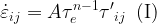
This equation is known as Nye’s generalization of Glen’s law, or Glen’s law for short. Much research has been devoted to the values of the rate factor A and the exponent n, and we should discuss them in some detail because these coefficients appear in the glacier profile equations. Factor A is closely related to temperature; indeed, for temperatures lower than 10^oC, the value of A has been associated to an Arrhenius-type law $\displaystyle A$ = $\displaystyle {{A}_{0}}\exp \left( {-{Q}/{{RT}}\;} \right)$ , where A₀ is the so-called pre-exponential factor, Q is the activation energy for creep, R is the gas constant, and T is temperature.

Laboratory experiments generally support values of n around 3 for effective stresses in the range of 200 to 2000 kPa, in agreement with theoretical considerations. At stresses more common in glaciers (<200 kPa), the exponent may be less than 3 (including n = 1, describing a Newtonian viscous fluid), but these experiments must be interpreted with caution due to the great difficulty in conducting such tests and because in many of the experiments the ice is deformed for only a limited time to strains of a few percent. Nevertheless, analysis of field data and laboratory experiments supports a transition from deformation at n $\displaystyle \approx$ 3 at high stresses to n $\displaystyle \le$ 2 at low stresses.

2. The parabolic glacier profile

A material exhibits perfect plasticity if deformation is negligible when the applied stress is below some critical value, the yield stress. For stresses larger than the yield stress, the material deforms “instantly” to relieve the applied stress. As a result, the stress in the material never exceeds the yield stress. For sufficiently large stresses, glacier flow may be treated as a problem in plasticity. In effect, this is equivalent to taking the limit n $\displaystyle \to$ $\displaystyle \infty$ for the exponent in the flow law. Making the perfect plasticity approximation allows the geometry of a glacier to be determined with a minimum of information, as we will see shortly. While this may not be realistic, it is often the best one can do, especially when reconstructing the large ice sheets that covered the American and European continents during the last glacial period.

Neglecting the effects of gradients in longitudinal stress and lateral drag, the driving stress is balanced by drag at the glacier bed, and the shear stress, $\displaystyle {{\tau }_{{xz}}}$ , increases linearly with depth from zero at the surface to the value of the basal drag at the bed. Assuming perfect plasticity, the stress in the ice cannot exceed the yield stress, $\displaystyle {{\tau }_{0}}$ , and basal drag must be equal to $\displaystyle {{\tau }_{0}}$ . Equating basal drag to the driving stress, which is assumed to be constant, we may write

$\displaystyle -\rho gH\frac{{\partial h}}{{\partial x}}={{\tau }_{0}}\,\,\,(\text{II})$

where $\displaystyle \rho$ is the density of ice, H is ice thickness, and h is surface elevation. Making the assumption that the glacier rests on a horizontal bed ( $\displaystyle \partial h/\partial x$ = $\displaystyle \partial H/\partial x$ ), the foregoing equation can be integrated to give

$\displaystyle -\rho gH\frac{{\partial H}}{{\partial x}}={{\tau }_{0}}$

$\displaystyle \therefore H\partial H=-\frac{{{{\tau }_{0}}}}{{\rho g}}\partial x$

$\displaystyle \therefore {{H}^{2}}=-\frac{{2{{\tau }_{0}}}}{{\rho g}}x+C$

The integration constant, C, can be determined from the condition that the ice thickness must be zero at the edge of the glacier, that is, H(L) = 0. Thus,

$\displaystyle C=\frac{{2{{\tau }_{0}}}}{{\rho g}}L$

so that

$\displaystyle {{H}^{2}}=-\frac{{2{{\tau }_{0}}}}{{\rho g}}x+\frac{{2{{\tau }_{0}}}}{{\rho g}}L$

$\displaystyle \therefore {{H}^{2}}=\frac{{2{{\tau }_{0}}}}{{\rho g}}\left( {L-x} \right)$

$\displaystyle \therefore H\left( x \right)={{\left[ {\frac{{2{{\tau }_{0}}}}{{\rho g}}\left( {L-x} \right)} \right]}^{{{1}/{2}\;}}}\,\,\,(\text{III})$

The thickness at the divide, H₀, is given by

$\displaystyle {{H}_{0}}={{\left( {\frac{{2{{\tau }_{0}}}}{{\rho g}}L} \right)}^{{{1}/{2}\;}}}\,\,\,(\text{IV})$

Accordingly, the profile of the plastic ice sheet is determined to be

$\displaystyle H\left( x \right)={{H}_{0}}{{\left( {1-\frac{x}{L}} \right)}^{{{1}/{2}\;}}}\,\,(\text{V})$

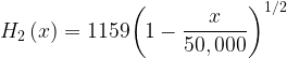
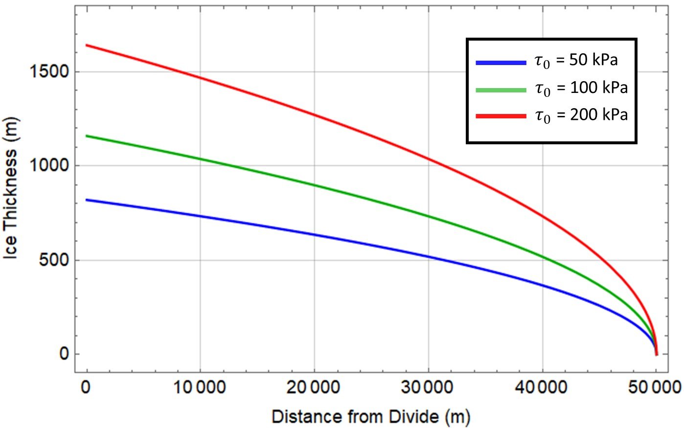
The elevation decreases parabolically toward the glacier edge; Considering a glacier of 100-km length, constituted of mineral ice of 910 kg/m³ density, we can readily use equation (V) to plot glacier profiles for different yield stresses. Suppose we had $\displaystyle {{\tau }_{0}}$ = 60 kPa, 120 kPa, and 240 kPa. For the first value,

$\displaystyle {{H}_{0}}={{\left( {\frac{{2\times 60,000}}{{910\times 9.81}}\times 10,000} \right)}^{{{1}/{2}\;}}}=820\,\text{m}$

so that the glacier profile can be described by

$\displaystyle {{H}_{1}}\left( x \right)=820{{\left( {1-\frac{x}{{50,000}}} \right)}^{{{1}/{2}\;}}}$

For $\displaystyle {{\tau }_{0}}$ = 120 kPa, in turn, we get H₀ = 1159 m and

$\displaystyle {{H}_{2}}\left( x \right)=1159{{\left( {1-\frac{x}{{50,000}}} \right)}^{{{1}/{2}\;}}}$

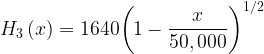
Finally, for $\displaystyle {{\tau }_{0}}$ = 240 kPa, we get H₀ = 1640 m and

$\displaystyle {{H}_{3}}\left( x \right)=1640{{\left( {1-\frac{x}{{50,000}}} \right)}^{{{1}/{2}\;}}}$

The three profiles are plotted below.

Equation (IV) gives the thickness of the central divide of a glacier or ice sheet. Cuffey and Paterson (2010) provide some interesting observations on the validity of this equation. As a first check, equation (IV), with $\displaystyle {{\tau }_{0}}$ = 100 kPa, can be applied to Greenland, giving H₀ = 3.15 km; this is close to the true value of about 3.2 km. For East Antarctica, using a typical dimension of L = 1000 km gives H₀ = 4.7 km. Although there are a few spots in Antarctica with ice this deep, it is too high as a typical value; most ice thicknesses along the central divides are in the range 3 to 4 km. Cuffey and Paterson then recommend using a different value of $\displaystyle {{\tau }_{0}}$ , in that driving stresses of 100 to 150 kPa, while reasonable for valley glaciers, are seemingly too high for ice sheets. Using a value $\displaystyle {{\tau }_{0}}$ = 75 kPa instead of 100 kPa in equation (IV) reduces H₀ by 14%. Though very rough, these calculations are still remarkable for their ability to explain a major characteristic of ice sheets from a single property of ice – yield strength – that can be easily measured from laboratory experiments.

3. The Vialov profile

In 1958, Vialov proposed an alternative expression to describe the profile of a glacier. His formulation applies to a glacier that flows by internal deformation only, over a flat bed and with constant rate of surface accumulation. The equation proposed by that researcher, often known as the Vialov profile, is

$\displaystyle {{\left[ {H\left( x \right)} \right]}^{{2+{2}/{n}\;}}}=K\left( {{{L}^{{1+{1}/{n}\;}}}-{{x}^{{1+{1}/{n}\;}}}} \right)\,\,(\text{VI})$

where

$\displaystyle K=\frac{{2{{{\left( {n+2} \right)}}^{{{1}/{n}\;}}}}}{{\rho g}}{{\left( {\frac{{{{w}_{s}}}}{{2A}}} \right)}^{{{1}/{n}\;}}}(\text{VII})$

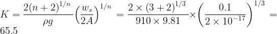
In these equations, A and n are parameters in Glen’s flow law, $\displaystyle \rho$ is the density of the ice, and w_s is the surface accumulation rate (which, again, should be constant). Let’s put the Vialov profile to use in an ice sheet such that n = 3, A = 10^-17 yr^-1Pa^-3, L = 500 km, w_s = 0.1 m/yr, and $\displaystyle \rho$ = 910 kg/m³. We begin by calculating K,

$\displaystyle K=\frac{{2{{{\left( {n+2} \right)}}^{{{1}/{n}\;}}}}}{{\rho g}}{{\left( {\frac{{{{w}_{s}}}}{{2A}}} \right)}^{{{1}/{n}\;}}}=\frac{{2\times {{{\left( {3+2} \right)}}^{{{1}/{3}\;}}}}}{{910\times 9.81}}\times {{\left( {\frac{{0.1}}{{2\times {{{10}}^{{-17}}}}}} \right)}^{{{1}/{3}\;}}}=65.5$

Then, we insert this value, along with L = 500,000 m and n = 3, into equation (VI),

$\displaystyle H\left( x \right)={{\left[ {65.5\times \left( {{{{500,000}}^{{1+1/3}}}-{{x}^{{1+1/3}}}} \right)} \right]}^{{{1}/{{\left( {2+2/3} \right)}}\;}}}$

$\displaystyle \therefore H\left( x \right)=4.80{{\left( {3.97\times {{{10}}^{7}}-{{x}^{{{4}/{3}\;}}}} \right)}^{{{3}/{8}\;}}}$

The Vialov profile in question is plotted below.

The Vialov profile has some important limitations, most of which are shared with the simple parabolic law. For one, at the divide (x = 0) the curvature of the profile is infinite, a problem related to the fact that the shallow ice approximation is not valid at that region. Further, the slope of the profile is infinite at the margins x = $\displaystyle \pm$ L, which violates the assumption of small surface slopes.

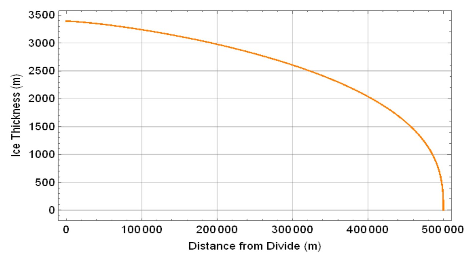
The volume flux for the Vialov profile is given by Q(x) = w_sx, with w_s = 0.1 m/yr. Plotting this simple equation for -500 km < x < +500 km should yield a straight line that crosses the origin at x = 0. At either margin, the volume flux reaches a maximum |Q(L)| = w_s|L| = 0.1 $\displaystyle \times$ 500,000 = 50,000 m²/yr, which can be interpreted as the calving rate into a surrounding ocean.

One important quantity that one can derive from the Vialov profile is the driving stress distribution, which is given by equation (II).

$\displaystyle {{\tau }_{b}}=-\rho gH\frac{{\partial H}}{{\partial x}}$

The derivative on the right-hand side can be obtained with any CAS package. We proceed to plot $\displaystyle {{\tau }_{d}}$ versus x, as shown.

Here we find yet another limitation of the Vialov profile: in the limit of x $\displaystyle \to$ L, the driving stress diverges, and basal shear stress is unbounded at the ice margin.

4. The Bueler profile

In the early 2000s, Bueler proposed a glacier profile model that improves on some of the shortcomings of the Vialov approach. The Bueler profile, as we might call it, is given by

$\displaystyle H\left( x \right)=\frac{{{{H}_{0}}}}{{{{{\left( {n-1} \right)}}^{{{n}/{{\left( {2n+2} \right)}}\;}}}}}{{\left[ {\left( {n+1} \right)\frac{x}{L}-n{{{\left( {\frac{x}{L}} \right)}}^{{{{\left( {n+1} \right)}}/{n}\;}}}+n{{{\left( {1-\frac{x}{L}} \right)}}^{{{{\left( {n+1} \right)}}/{n}\;}}}-1} \right]}^{{{n}/{{\left( {2n+2} \right)}}\;}}}\,\,\,(\text{VIII})$

where H₀, the surface elevation at the ice divide, is given by

$\displaystyle H_{0}^{{{{\left( {2n+2} \right)}}/{n}\;}}=2L{{\left( {\frac{\alpha }{{{{A}_{0}}}}} \right)}^{{{1}/{n}\;}}}\left( {\frac{{n-1}}{n}} \right)\,\,\,(\text{IX})$

Here, $\displaystyle \alpha$ is an adjustable parameter and A₀ is such that

$\displaystyle {{A}_{0}}=\frac{{2A{{{\left( {\rho g} \right)}}^{n}}}}{{n+2}}\,\,\,(\text{X})$

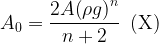
Let’s find a Bueler curve that fits the data given in the previous section. We begin by computing A₀,

$\displaystyle {{A}_{0}}=\frac{{2\times {{{10}}^{{-17}}}\times {{{\left( {910\times 9.81} \right)}}^{3}}}}{{3+2}}=2.85\times {{10}^{{-6}}}$

Notice that we have ignored the units of A₀ for convenience. Then, substituting into equation (IX) brings to

$\displaystyle {{H}_{0}}={{\left[ {2\times 500,000\times {{{\left( {\frac{\alpha }{{2.85\times {{{10}}^{{-6}}}}}} \right)}}^{{{1}/{3}\;}}}\times \left( {\frac{{3-1}}{3}} \right)} \right]}^{{{1}/{{\left[ {\left( {2\times 3+2/3} \right)} \right]}}\;}}}=754{{\alpha }^{{{1}/{8}\;}}}$

To fit equation (VIII) to a Bueler profile using Mathematica, we first compute some data with the Vialov profile obtained in the previous section,

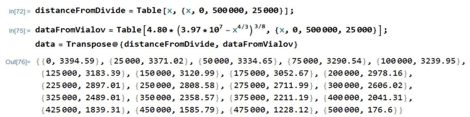
Then, we use FindFit,

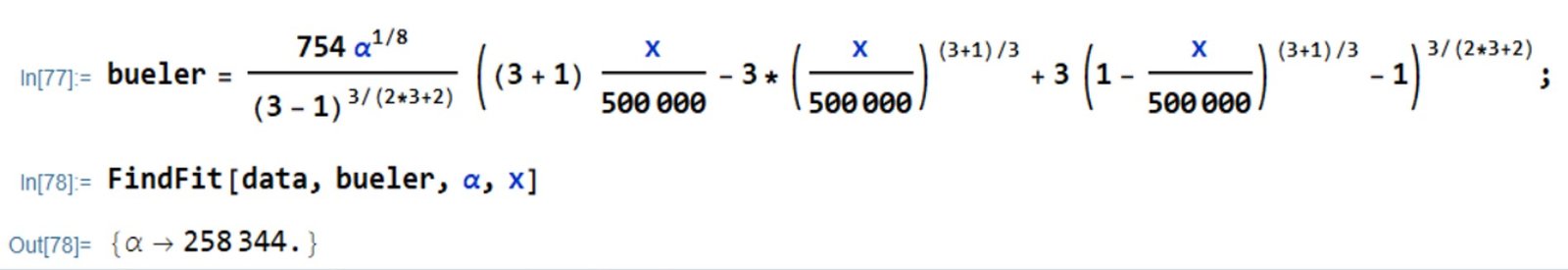
Clearly, we should obtain a Bueler profile similar to the Vialov profile produced in the previous section if we take $\displaystyle \alpha$ $\displaystyle \approx$ 258,340. Substituting into equation (VIII) brings to

$\displaystyle H\left( x \right)=\frac{{754\times {{{\left( {258,340} \right)}}^{{{1}/{8}\;}}}}}{{{{{\left( {3-1} \right)}}^{{{3}/{{\left( {2\times 3+2} \right)}}\;}}}}}{{\left[ {\left( {3+1} \right)\frac{x}{{500,000}}-3{{{\left( {\frac{x}{{500,000}}} \right)}}^{{{{\left( {3+1} \right)}}/{3}\;}}}+3{{{\left( {1-\frac{x}{{500,000}}} \right)}}^{{{{\left( {3+1} \right)}}/{3}\;}}}-1} \right]}^{{{3}/{{\left( {2\times 3+2} \right)}}\;}}}$

This thickness distribution is plotted along with the Vialov profile obtained in the previous section; the orange curve is the Vialov profile and the purple curve is the Bueler profile.

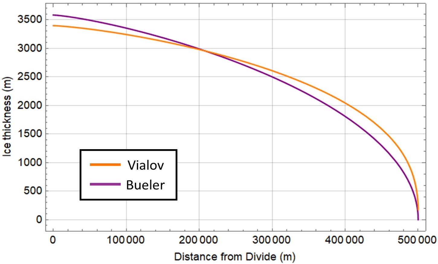
Notice that there is little difference between the two profiles, and the Bueler profile retains the undesired slope/curvature issues of the Vialov approach. Was the extra algebraic complexity of the former for nothing? Not at all. For starters, the Bueler profile corresponds to a volume flux equation,

$\displaystyle Q\left( x \right)=\alpha {{\left[ {{{{\left( {\frac{x}{L}} \right)}}^{{{1}/{n}\;}}}+{{{\left( {1-\frac{x}{L}} \right)}}^{{{1}/{n}\;}}}-1} \right]}^{n}}\,\,\,(\text{XI})$

that fulfills the symmetry condition Q(0) = 0 at the ice divide and the no-flux condition Q(L) = 0 at the margin. Q(x) for the data at hand is plotted below.

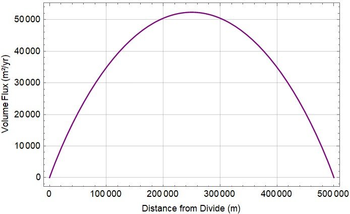
Deriving the volume flux should give the mass balance function,

$\displaystyle {{w}_{s}}\left( x \right)=\frac{{dQ}}{{dx}}=\frac{\alpha }{L}{{\left[ {{{{\left( {\frac{x}{L}} \right)}}^{{{1}/{n}\;}}}+{{{\left( {1-\frac{x}{L}} \right)}}^{{{1}/{n}\;}}}-1} \right]}^{{\left( {n-1} \right)}}}\times \left[ {{{{\left( {\frac{x}{L}} \right)}}^{{{{\left( {1-n} \right)}}/{n}\;}}}-{{{\left( {1-\frac{x}{L}} \right)}}^{{{{\left( {1-n} \right)}}/{n}\;}}}} \right]\,\,(\text{XII})$

which is plotted below for the data we were given. The surface mass balance is positive (accumulation) in the interior, high-elevation part of the ice sheet and negative (ablation) in the low-elevation part near the margin. An unrealistic feature is the steep increase towards the ice divide.

It remains to plot the distribution of basal shear stress (driving stress) for the Bueler profile. To do so, we substitute H(x) from (VIII) into equation (II); the derivative dH/dx can be obtained with any CAS. We also replot the stress distribution obtained from the Vialov profile.

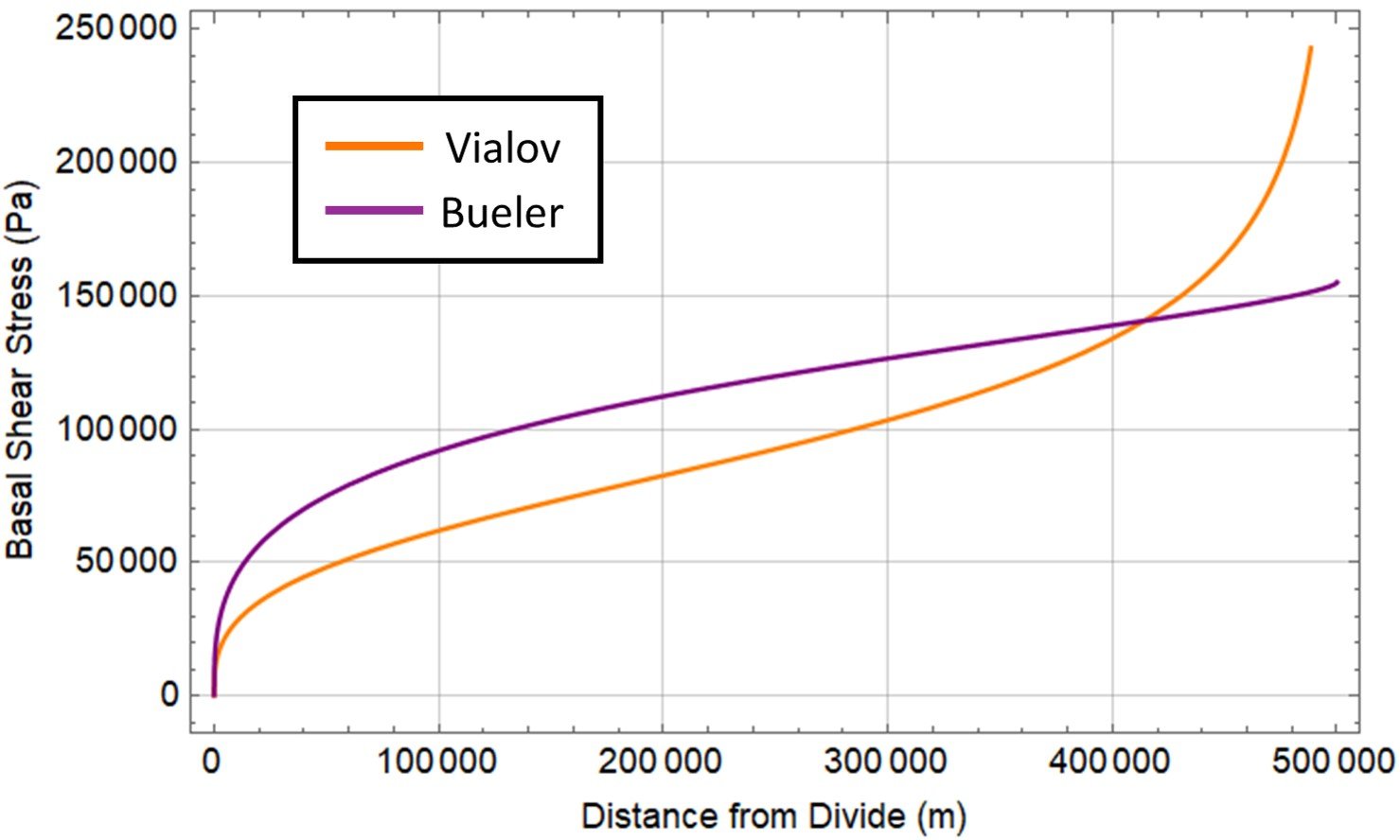
Unlike basal shear in the Vialov profile, which surges close to the margin, $\displaystyle {{\tau }_{d}}$ in the Bueler model increases steadily as one moves away from the divide, becoming indeterminate only when we are very close to x = L.

References

• CUFFEY, K. and PATERSON, W. (2010). The Physics of Glaciers. 4th edition. Oxford: Butterworth-Heinemann.

• GREVE, R. and BLATTER, H. (2009). Dynamics of Ice Sheets and Glaciers. Berlin/Heidelberg: Springer.

• VAN DER VEEN, C. (2013). Fundamentals of Glacier Dynamics. 2nd edition. Boca Raton: CRC Press.

• Van der Veen, C. and Whillans, I. (1990). Flow laws for glacier ice: comparison of numerical predictions and field measurements. Journal of Glaciology, 36(124): 324 – 339.

Glacier Profiles: The Parabolic, Vialov, and Bueler Models

Subscribe to our Mailing List!

Featured Posts

A Primer on NAND Flash Memories

Solidification Time and Chvorinov’s Rule

Step-Growth Polymerization, the Carothers Equation, and the Flory-Schulz Distribution

More Articles

Bagnold’s Blown Sand Transport and Saltation

Air Pollution and the Gaussian Plume Model

Fields of Study

More

© 2024 Montogue Quiz

Subscribe to
our Mailing List!

Subscribe to our Mailing List!

Subscribe to receive our latest materials in your inbox.

Homework Help

© 2024 Montogue Quiz

Subscribe to our Mailing List!