

In this article, I apply basic math to derive some interesting results on the geodynamics of oceanic and continental lithosphere. In section 1, I use the half-space model to derive relations for the geothermal flow and depth of the seafloor. In section 2, I introduce McKenzie’s model of subsidence and include a simple spreadsheet that readers are free to play around with. Finally, section 3 is dedicated to continental lithosphere and the concept of heat flow province, which I illustrate with a solved example.
1. Heat flow and oceanic depth
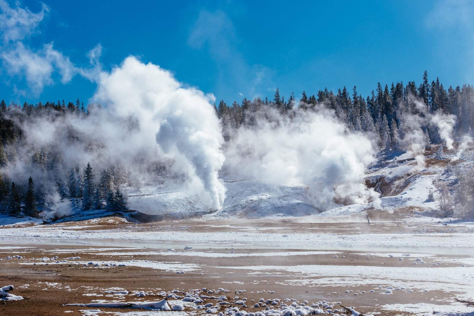
Thermal conditions of an oceanic plate are different from those of a continental plate, because the material cools as it moves away from the ridge and the radiogenic heat in the crust is negligible. The simplest thermal model of oceanic lithosphere is to consider a semi-infinite half-space. If x and z are the horizontal and vertical coordinates, respectively, and v = dx/dt denotes the plate velocity, assumed to be constant and in practice determined by the age t of the crust at a distance x from the ridge, we may write
Further, if horizontal heat conduction is negligible compared to heat conduction by the plate’s vertical motion, the Laplacian of temperature can be simplified as

It follows that the Fourier equation simplifies to

where 
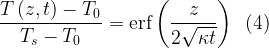
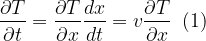
where erf denotes the Gaussian error function. Equation (4) provides the temperature distribution along the plate with age. One immediate application of this result is the calculation of the geothermal flow q0. Rearranging (4) gives
where u = z/(4

Noting that geothermal flow equals the product of thermal conductivity and geothermal gradient, it follows that, with z = 0,

This result shows that, except for factor 


Figure 1. Geothermal heat flow perpendicular to ridge as a function of age. The solid curve is equation (7) and the data points are taken from Stein and Stein (1992).
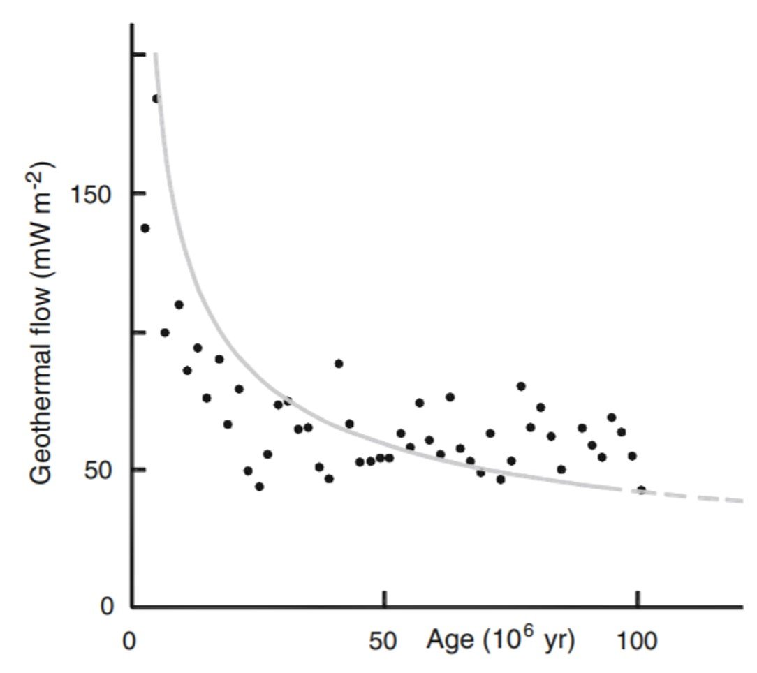
Note that an undesirable feature of equation (7) is that it yields an infinite heat flux at t = 0. A simple workaround would be to use the total heat H instead; H is given by integrating q0 from t = 0 to t,

In the mid-1800s, William Thompson, later Lord Kelvin, used the theory for the conductive cooling of a semi-infinite half-space to estimate the age of the Earth. He hypothesized that the Earth was formed at a uniform temperature T1 and that its surface was subsequently maintained at a low temperature T0. He assumed that a thin near-surface boundary layer developed as the Earth cooled. Since the boundary layer would be thin compared with the radius of the Earth, he reasoned that the one-dimensional model developed in this section could be applied. Using an equation similar to (7), he concluded that the age of the Earth t0 was given by


where dT/dz is the present near-surface thermal gradient. With dT/dz = 25 K/km, T1 – T0 = 2000 K, and
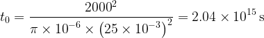
or approximately 65 million years. One of the reasons why this approximation misses the real value of 4.54 billion years by such a large margin is that it does not account for radiogenic heat. It was not until radioactivity was discovered at about 1900 that Kelvin’s estimate was seriously questioned.
Since the oceanic lithosphere is approximately in isostatic equilibrium, the average seafloor depth should increase with age as a consequence of the density increase caused by cooling. The principle of isostasy states that there is the same mass per unit area between the surface and the depth of compensation for any vertical column of material. Thus, by denoting with hw the depth of the ocean floor, hl and 


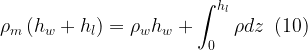
or

where 

so that, substituting in (11), we have

Substituting the temperature profile from (7), we write
![\displaystyle {{h}_{w}}\left( {{{\rho }_{m}}-{{\rho }_{w}}} \right)=\alpha {{\rho }_{m}}\left( {{{T}_{s}}-{{T}_{0}}} \right)\int_{0}^{\infty }{{\left[ {\text{erfc}\left( {\frac{z}{{2\sqrt{{\kappa t}}}}} \right)} \right]dz}}\,\,\,(14)](https://s0.wp.com/latex.php?latex=%5Cdisplaystyle+%7B%7Bh%7D_%7Bw%7D%7D%5Cleft%28+%7B%7B%7B%5Crho+%7D_%7Bm%7D%7D-%7B%7B%5Crho+%7D_%7Bw%7D%7D%7D+%5Cright%29%3D%5Calpha+%7B%7B%5Crho+%7D_%7Bm%7D%7D%5Cleft%28+%7B%7B%7BT%7D_%7Bs%7D%7D-%7B%7BT%7D_%7B0%7D%7D%7D+%5Cright%29%5Cint_%7B0%7D%5E%7B%5Cinfty+%7D%7B%7B%5Cleft%5B+%7B%5Ctext%7Berfc%7D%5Cleft%28+%7B%5Cfrac%7Bz%7D%7B%7B2%5Csqrt%7B%7B%5Ckappa+t%7D%7D%7D%7D%7D+%5Cright%29%7D+%5Cright%5Ddz%7D%7D%5C%2C%5C%2C%5C%2C%2814%29&bg=ffffff&fg=000&s=1&c=20201002)
where we have changed the upper bound of the integral from z = hl to z = 


Here, we appeal to the standard result
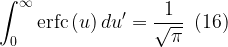
so that
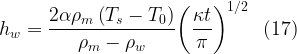
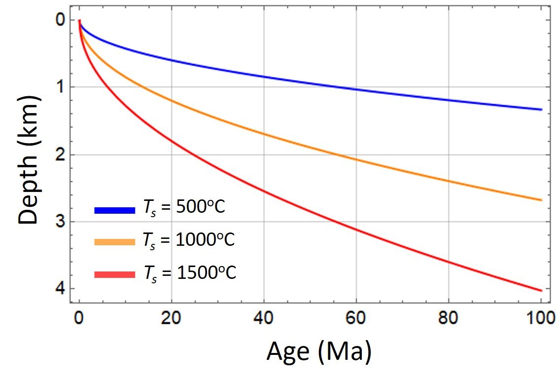
This expression shows that, if isostatic conditions prevail, the average depth of the ocean will increase with the square root of age. Figure 2 plots equation (17) for three temperatures Ts = 500oC, 1000oC, and 1500oC.
Figure 2. Evolution of oceanic depth given by equation (17) for for three temperatures Ts. Values used were 
2. McKenzie’s (1978) subsidence model
McKenzie (1978) used the observations of the deep structure of rift-type basins together with the exponential nature of their subsidence to suggest a kinematic model for rift-type basin evolution, which predicts subsidence and uplift, crustal thinning, and heat flow for different times since rifting. He showed that, as a consequence of extension, there is an initial subsidence due to crustal thinning followed by a thermal subsidence as the stretched lithosphere cools. Consider some initial thickness of the crust, tc, and lithosphere, a, a steady-state geothermal gradient in the lithosphere (which includes the crust) and an isothermal sub-lithospheric mantle. If the temperature at the surface of the lithosphere is 0oC and the temperature at its base is T1, then the average temperature at the base of the crust is given by

Similarly, the average temperature in the sub-crustal mantle is

The pressure at the base of the unstretched column is given by

where
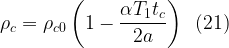
![\displaystyle {{\rho }_{l}}={{\rho }_{{l0}}}\left[ {1-\frac{{\alpha {{T}_{1}}\left( {{{t}_{c}}+a} \right)}}{{2a}}} \right]\,\,\,(22)](https://s0.wp.com/latex.php?latex=%5Cdisplaystyle+%7B%7B%5Crho+%7D_%7Bl%7D%7D%3D%7B%7B%5Crho+%7D_%7B%7Bl0%7D%7D%7D%5Cleft%5B+%7B1-%5Cfrac%7B%7B%5Calpha+%7B%7BT%7D_%7B1%7D%7D%5Cleft%28+%7B%7B%7Bt%7D_%7Bc%7D%7D%2Ba%7D+%5Cright%29%7D%7D%7B%7B2a%7D%7D%7D+%5Cright%5D%5C%2C%5C%2C%5C%2C%2822%29&bg=ffffff&fg=000&s=1&c=20201002)
and 

![\displaystyle {{\rho }_{{c0}}}\left( {1-\frac{{\alpha {{T}_{1}}{{t}_{c}}}}{{2a}}} \right)g{{T}_{c}}+{{\rho }_{{l0}}}\left[ {1-\frac{{\alpha {{T}_{1}}\left( {{{t}_{c}}+a} \right)}}{{2a}}} \right]g\left( {a-{{t}_{c}}} \right)\,\,\,(23)](https://s0.wp.com/latex.php?latex=%5Cdisplaystyle+%7B%7B%5Crho+%7D_%7B%7Bc0%7D%7D%7D%5Cleft%28+%7B1-%5Cfrac%7B%7B%5Calpha+%7B%7BT%7D_%7B1%7D%7D%7B%7Bt%7D_%7Bc%7D%7D%7D%7D%7B%7B2a%7D%7D%7D+%5Cright%29g%7B%7BT%7D_%7Bc%7D%7D%2B%7B%7B%5Crho+%7D_%7B%7Bl0%7D%7D%7D%5Cleft%5B+%7B1-%5Cfrac%7B%7B%5Calpha+%7B%7BT%7D_%7B1%7D%7D%5Cleft%28+%7B%7B%7Bt%7D_%7Bc%7D%7D%2Ba%7D+%5Cright%29%7D%7D%7B%7B2a%7D%7D%7D+%5Cright%5Dg%5Cleft%28+%7Ba-%7B%7Bt%7D_%7Bc%7D%7D%7D+%5Cright%29%5C%2C%5C%2C%5C%2C%2823%29&bg=ffffff&fg=000&s=1&c=20201002)
The effect of rifting is to thin the crust and lithosphere and to raise the geotherm. We can write the thickness of the thinned crust as tc/
![\displaystyle {{\rho }_{w}}{{S}_{i}}g+{{\rho }_{{c0}}}\left( {1-\frac{{\alpha {{T}_{1}}{{t}_{c}}}}{{2a}}} \right)g\frac{{{{t}_{c}}}}{{{{\beta }_{s}}}}+{{\rho }_{{l0}}}\left[ {1-\frac{{\alpha {{T}_{1}}\left( {{{t}_{c}}+a} \right)}}{{2a}}} \right]g\left( {\frac{a}{{{{\beta }_{s}}}}-\frac{{{{t}_{c}}}}{{{{\beta }_{s}}}}} \right)+{{\rho }_{{l0}}}\left( {1-\alpha {{T}_{1}}} \right)g\left( {a-{{S}_{i}}-\frac{a}{{{{\beta }_{s}}}}} \right)\,\,\,(24)](https://s0.wp.com/latex.php?latex=%5Cdisplaystyle+%7B%7B%5Crho+%7D_%7Bw%7D%7D%7B%7BS%7D_%7Bi%7D%7Dg%2B%7B%7B%5Crho+%7D_%7B%7Bc0%7D%7D%7D%5Cleft%28+%7B1-%5Cfrac%7B%7B%5Calpha+%7B%7BT%7D_%7B1%7D%7D%7B%7Bt%7D_%7Bc%7D%7D%7D%7D%7B%7B2a%7D%7D%7D+%5Cright%29g%5Cfrac%7B%7B%7B%7Bt%7D_%7Bc%7D%7D%7D%7D%7B%7B%7B%7B%5Cbeta+%7D_%7Bs%7D%7D%7D%7D%2B%7B%7B%5Crho+%7D_%7B%7Bl0%7D%7D%7D%5Cleft%5B+%7B1-%5Cfrac%7B%7B%5Calpha+%7B%7BT%7D_%7B1%7D%7D%5Cleft%28+%7B%7B%7Bt%7D_%7Bc%7D%7D%2Ba%7D+%5Cright%29%7D%7D%7B%7B2a%7D%7D%7D+%5Cright%5Dg%5Cleft%28+%7B%5Cfrac%7Ba%7D%7B%7B%7B%7B%5Cbeta+%7D_%7Bs%7D%7D%7D%7D-%5Cfrac%7B%7B%7B%7Bt%7D_%7Bc%7D%7D%7D%7D%7B%7B%7B%7B%5Cbeta+%7D_%7Bs%7D%7D%7D%7D%7D+%5Cright%29%2B%7B%7B%5Crho+%7D_%7B%7Bl0%7D%7D%7D%5Cleft%28+%7B1-%5Calpha+%7B%7BT%7D_%7B1%7D%7D%7D+%5Cright%29g%5Cleft%28+%7Ba-%7B%7BS%7D_%7Bi%7D%7D-%5Cfrac%7Ba%7D%7B%7B%7B%7B%5Cbeta+%7D_%7Bs%7D%7D%7D%7D%7D+%5Cright%29%5C%2C%5C%2C%5C%2C%2824%29&bg=ffffff&fg=000&s=0&c=20201002)
where Si is initial subsidence and
![\displaystyle {{S}_{i}}=\frac{{a\left[ {\left( {{{\rho }_{{l0}}}-{{\rho }_{{co}}}} \right)\frac{{{{t}_{c}}}}{a}\left( {1-\frac{{\alpha {{T}_{1}}{{t}_{c}}}}{{2a}}} \right)-\frac{{{{\rho }_{{l0}}}\alpha {{T}_{1}}}}{2}} \right]\left( {1-\frac{1}{{{{\beta }_{s}}}}} \right)}}{{{{\rho }_{{l0}}}\left( {1-\alpha {{T}_{1}}} \right)-{{\rho }_{w}}}}\,\,\,(25)](https://s0.wp.com/latex.php?latex=%5Cdisplaystyle+%7B%7BS%7D_%7Bi%7D%7D%3D%5Cfrac%7B%7Ba%5Cleft%5B+%7B%5Cleft%28+%7B%7B%7B%5Crho+%7D_%7B%7Bl0%7D%7D%7D-%7B%7B%5Crho+%7D_%7B%7Bco%7D%7D%7D%7D+%5Cright%29%5Cfrac%7B%7B%7B%7Bt%7D_%7Bc%7D%7D%7D%7D%7Ba%7D%5Cleft%28+%7B1-%5Cfrac%7B%7B%5Calpha+%7B%7BT%7D_%7B1%7D%7D%7B%7Bt%7D_%7Bc%7D%7D%7D%7D%7B%7B2a%7D%7D%7D+%5Cright%29-%5Cfrac%7B%7B%7B%7B%5Crho+%7D_%7B%7Bl0%7D%7D%7D%5Calpha+%7B%7BT%7D_%7B1%7D%7D%7D%7D%7B2%7D%7D+%5Cright%5D%5Cleft%28+%7B1-%5Cfrac%7B1%7D%7B%7B%7B%7B%5Cbeta+%7D_%7Bs%7D%7D%7D%7D%7D+%5Cright%29%7D%7D%7B%7B%7B%7B%5Crho+%7D_%7B%7Bl0%7D%7D%7D%5Cleft%28+%7B1-%5Calpha+%7B%7BT%7D_%7B1%7D%7D%7D+%5Cright%29-%7B%7B%5Crho+%7D_%7Bw%7D%7D%7D%7D%5C%2C%5C%2C%5C%2C%2825%29&bg=ffffff&fg=000&s=1&c=20201002)
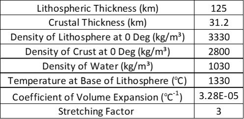
This equation gives the initial subsidence for different values of initial thickness, temperature, density of crust and sub-crustal mantle, and stretching factor. This is a lengthy formula, so I’ve set up a simple spreadsheet to automate calculations; download it here. Using the sample values listed in Table 1, the spreadsheet returns densities 

Table 1. Data for sample subsidence calculations
The final subsidence can be obtained by balancing the pressure at the base of the unstretched column with the final column. The pressure at the base of the unstretched column is given by (23). The pressure at the base of the final column is, in turn,
where 


where

Using the same parameters as before, we obtain
The thermal subsidence, 

Substituting the values for Si and Sf above gives

Since the temperature distribution determines the density structure, equation (3) can be used to calculate subsidence as a function of time. The elevation e(t) above the final depth to which the lithosphere (which includes the crust) sinks is given, for example, by McKenzie (1978), who proposed

where
and
The thermal subsidence,

where

A plot of 
3. Continental lithosphere and heat flow provinces
Continental heat flow is harder to understand than oceanic heat flow and harder to fit into a general theory of thermal evolution of the continents or of the Earth. Continental heat-flow values are affected by many factors, including erosion, deposition, glaciation, the length of time since any tectonic events, local concentrations of heat-generating elements in the crust, the presence or absence of aquifers and the drilling of the hole in which the measurements were made. Nevertheless, it is clear that the measured heat-flow values decrease with increasing age. This suggests that, like the oceanic lithosphere, continental lithosphere is cooling and slowly thickening with time.
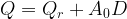
In some specific areas, there is a linear relationship between surface heat flow and surface radioactive heat generation. Using this relationship, one can make an approximate estimate of the contribution of the heat-generating elements in the continental crust to the surface heat flow. In these areas, the surface heat flow Q0 can be expressed in terms of the measured surface radioactive heat generation A0 as

where Qr is a constant component of heat flow from the mantle and D represents a depth scale for the vertical distribution of heat-producing elements. A reliable consistency in parameter D at some interval of depths, typically between 10 and 15 km, led workers to define a heat flow province as a region of common tectonothermal history within which consistent values of Qr and D are obtained. Much effort has been expended in identifying and quantifying heat flow provinces around the world. Several regional correlations are given in Figure 3. In each case, the corresponding length scale D is the slope of the best-fit straight line and the reduced heat flow Qr is the vertical intercept of the line. These data are summarized in Table 2. Note that in each case a linear correlation appears to fit the data quite well. In all cases the length scale is near 10 km and the reduced heat flow Qr in general appears to be consistent with the range quoted in Pasquale et al. (2014), who suggest Qr values ranging from 18 mW/m2 for Precambrian areas to 45 mW/m2 for Cenozoic areas.
Figure 3. Dependence of surface heat flow Q0 on radiogenic heat production A0 per unit volume in surface rock for selected geological provinces: Sierra Nevada (solid squares and very long dashed line), eastern US (solid circles and intermediate dashed line), Norway and Sweden (open circles and solid line), eastern Canadian shield (open squares and short dashed line). In each case the data are fit with the linear relationship (36).
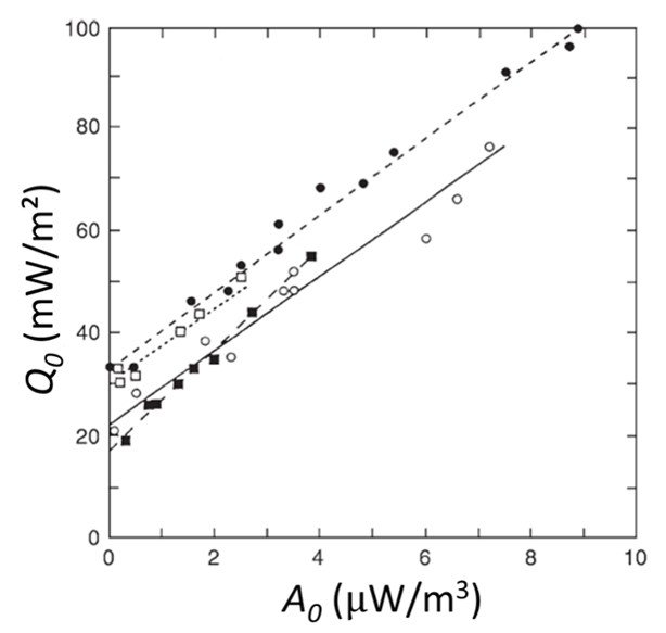
Table 2. Coefficients for linear fit equations shown in Figure 3.

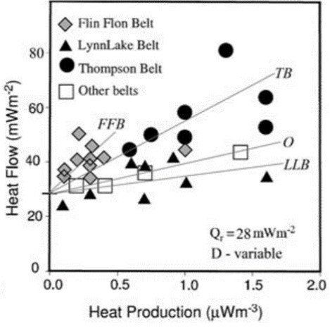
Although equation (36) provides a convenient, simplified description of the thermal structure of continental lithosphere, several objections have been raised over its validity in specific situations. For one, models involving heat-flow provinces often lump together regions and belts with clearly distinct origins and lithologies. Artemieva (2011) mentions the Paleoproterozoic Trans-Hudson Orogen (the central Canadian shield) as an example. The orogen is formed by markedly different structures: the Flin Flon Belt is made up of arc volcanic and plutonic rocks; the Lynn Lake Belt is formed by island arc volcanic rocks; the Thompson Nickel Belt contains metasedimentary rocks; other domains are made up of Archean gneisses. While a single correlation could be suggested for the entire orogen, heat data gathered for individual regions suggest that at least parameter D should be treated as variable from one belt to the next, as illustrated in Figure 4.
Figure 4. Heat-flow province fits for regions of the central Canadian shield.
The second main issue in the heat-province linear equation concerns the fact that it is an effectively 1D treatment and that the scatter around data is, in part, caused by 2D and 3D heat flow effects that smooth lateral variations in heat production. The effect of horizontal variations in heat production in the crust on surface heat flow and thus on the Q–A0 relationship was examined by harmonic (Jaupart, 1983) and random (Vasseur and Singh, 1986) lateral distributions of heat sources in the crust with a constant or exponential vertical distribution. Those workers found that, in general, lateral flow smoothes variations in heat production so that only shallow anomalies are well reflected in surface heat flow. In almost all cases, lateral heat flow results in an apparently lower D-value as obtained from the heat flow-heat production plot than the actual thickness of the radioactive layer. The amplitude of this reduction depends on the radial distance over which the (randomly distributed) heat production is correlated. If the thickness of the radioactive D-layer is much smaller than the scale of horizontal fluctuations in radioactivity, vertical heat flow prevails and the effect of lateral heat production heterogeneity on Q and on the linear correlation (36) is insignificant. If, however, the scale of horizontal fluctuations is small compared to D, the contribution of lateral heat flow to surface heat flow variations becomes important (Vasseur and Singh, 1986).
Let’s close this article with a simple applied example.
Example
Suppose that, in the eastern United States, a heat flow province can be represented by the usual equation
Data from the US Geological Survey suggest that the local lithosphere can be approximated by a heat flow province equation with constants Qr = 34 mW/m2 and D = 7.2 km. Assuming a simple, steady-state, two-layer model of heat production, an average surface temperature of 12oC, an average thermal conductivity of 2.8 W/mK, and a measured surface heat generation of 3.2 W/m3, what is the temperature, T, at the base of the heat-generation layer?
The linear relationship tells us that surface heat flow

and the two-layer model tells us that heat flow decreases linearly with depth to Qr = 34 mW/m2 at 7.2 km. The thermal gradient (

As a boundary condition, T(0) = 12oC, giving


Finally, the temperature profile is given by

and the temperature at z = 7.2 km is

References
• ARTEMIEVA, I. (2011). The Lithosphere: An Interdisciplinary Approach. Cambridge: Cambridge University Press.
• BEARDSMORE, G. and CULL, J. (2001). Crustal Heat Flow. Cambridge: Cambridge University Press.
• Jaupart, C. (1983). Horizontal heat transfer due to radioactivity contrasts: causes and consequences of the linear heat flow relation. Geophys. J. Roy. Astron. Soc., 75, 411 – 435.
• McKenzie, D. (1978). Some remarks on the development of sedimentary basins. Earth Planet. Sci. Lett., 40, 25 – 32.
• PASQUALE, V., VERDOYA, M. and CHIOZZI, P. (2014). Geothermics: Heat Flow in the Lithosphere. Berlin/Heidelberg: Springer.
• Stein, C. and Stein, S. (1992). A model for the global variation in oceanic depth and heat flow with lithospheric age. Nature, 359, 123 – 128.

