Vorticity, Circulation, and Potential Vorticity

Many large-scale flows, especially those of meteorological and oceanographic interest, are rotational in nature. In this blog post, we discuss powerful conservation principles that greatly simplify the analysis of geophysical flows. Two solved examples are included along the way.

1. Introduction to vorticity

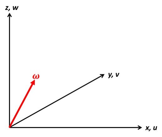
The vorticity vector of a flow described by Cartesian velocity components (u, v, w) (Figure 1) is denoted by the Greek letter $\displaystyle \mathbf{\omega }$ (omega) and can be stated as

$\displaystyle \mathbf{\omega }=\nabla \times \mathbf{u}=\left( {\frac{{\partial w}}{{\partial y}}-\frac{{\partial v}}{{\partial z}}} \right)\mathbf{i}+\left( {\frac{{\partial u}}{{\partial z}}-\frac{{\partial w}}{{\partial x}}} \right)\mathbf{j}+\left( {\frac{{\partial v}}{{\partial x}}-\frac{{\partial u}}{{\partial y}}} \right)\mathbf{k}\,\,\,(1)$

It expresses the local whirling rate of the fluid with both a magnitude and a spatial orientation. The vorticity observed from an inertial, nonrotating frame is called the absolute vorticity, $\displaystyle {{\mathbf{\omega }}_{a}}$ . In geophysical flows, absolute vorticity is usually divided into two components in accordance with the relation

$\displaystyle {{\mathbf{\omega }}_{a}}=\mathbf{\omega }+2\mathbf{\Omega }\,\,\,(2)$

Here, $\displaystyle \mathbf{\omega }$ is the relative vorticity, that is, the curl of relative velocity, and 2 $\displaystyle \mathbf{\Omega }$ is the planetary vorticity, that is, the contribution to vorticity due to rotation of the Earth. Following Pedlosky (1987), the relative magnitudes of these two components can be estimated in a preliminary manner as follows. The component of the planetary vorticity normal to the Earth’s surface is the so-called Coriolis parameter f,

$\displaystyle f=2\Omega \sin \phi \,\,\,(3)$

where $\displaystyle \mathbf{\Omega }$ $\displaystyle \approx$ 7.3 $\displaystyle \times$ 10^-5 rad/s is the rotational frequency of the Earth and $\displaystyle \phi$ is the latitude of the fluid element in question. The corresponding scalíng for the vertical component of the relative vorticity is given by the characteristic value of the velocity tangent to the Earth surface (the horizontal velocity) divided by the length scale L, that is,

$\displaystyle {{\omega }_{n}}=O\left( {\frac{U}{L}} \right)\,\,\,(4)$

The ratio of $\displaystyle {{\omega }_{n}}$ to f is then

$\displaystyle \frac{{{{\omega }_{n}}}}{f}=\frac{U}{{fL}}=\frac{U}{{2\Omega L\sin \phi }}=\text{R}{{\text{o}}_{L}}\,\,\,(5)$

where Ro_L is the local Rossby number, which expresses the ratio of the characteristic (inertial) velocity of the flow to the velocity induced by the Coriolis acceleration. In regions excluding the equator, sin $\displaystyle \phi$ is of the order of unity, so that low-Rossby number flows have the property that their relative vorticity is small compared to the planetary vorticity. This implies that large-scale flows such as those of interest to meteorologists and oceanographers are hardly ever free of vorticity, and that their vorticity primarily stems from planetary vorticity.

Figure 1. The vorticity vector.

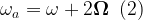
The typical values of vorticity in a large-scale flow in the extratropical atmosphere are v_z + w_y $\displaystyle \approx$ –v_z $\displaystyle \sim$ 10^-3 s^-1, u_z – w_x $\displaystyle \approx$ u_z $\displaystyle \sim$ 10^-3 s^-1, v_x – u_y $\displaystyle \sim$ 10^-5 s^-1. That is, the horizontal components of vorticity are typically two orders of magnitude larger than the vertical component. Although the vertical component is the smallest of the three, it has special significance for large-scale flows because such flows are quasi-horizontal and their fluctuation with respect to depth/altitude would give a clear indication of how the oceanic current/wind field is changing. This is why meteorologists and oceanographers often give particular importance to vertical vorticity. Unless specified otherwise, when scientists use the word “vorticity” and employ the symbol $\displaystyle \zeta$ (zeta), they are generally referring to the vertical component of the relative vorticity vector. Regions of large positive (negative) $\displaystyle \zeta$ tend to develop in association with cyclonic storms in the Northern (Southern) Hemisphere. Thus, the distribution of relative vorticity is an excellent diagnostic for weather analysis (Holton, 1992).

2. The vorticity equation

Replacing velocity with vorticity in the Navier-Stokes equations and employing the appropriate vector identities, we obtain the equation

$\displaystyle \frac{{\partial \mathbf{\omega }}}{{\partial t}}+\nabla \times \left( {{{\mathbf{\omega }}_{a}}\times \mathbf{u}} \right)=-\nabla \times \frac{1}{\rho }\nabla p+v{{\nabla }^{2}}\mathbf{\omega }\,\,\,(6)$

where $\displaystyle \mathbf{\omega }$ is relative vorticity, $\displaystyle {{\mathbf{\omega }}_{a}}$ is absolute vorticity, u is the velocity vector, $\displaystyle \rho$ is density, p is pressure, $\displaystyle \nu$ is kinematic viscosity, and t is time. Equation (6) is the general vorticity equation. A more convenient form of it is

$\displaystyle \frac{{D{{\mathbf{\omega }}_{a}}}}{{Dt}}={{\mathbf{\omega }}_{a}}\cdot \nabla \mathbf{u}-{{\mathbf{\omega }}_{a}}\nabla \cdot \mathbf{u}+\frac{1}{{{{\rho }^{2}}}}\nabla \rho \times \nabla p+v{{\nabla }^{2}}{{\mathbf{\omega }}_{a}}\,\,\,(7)$

As can be seen, the variation of absolute vorticity, expressed by the material derivative on the left-hand side, is made up of the four contributions on the right-hand side. If all terms on the right-hand side vanish, absolute vorticity is conserved. Considering each term individually, we have:

1. Vorticity diffusion term, $\displaystyle v{{\nabla }^{2}}{{\mathbf{\omega }}_{a}}$ . Considering this term individually, (7) could be restated as

$\displaystyle \frac{{\partial {{\zeta }_{a}}}}{{\partial t}}=v{{\nabla }^{2}}{{\zeta }_{a}}\,\,\,(8)$

which is akin to Fick’s second law of diffusion in mass transfer problems. Hence, this term represents vorticity diffusion due to internal (viscous) friction. In many geophysical flows, this term is the most obvious contribution to vorticity.

2. Tipping and stretching term, $\displaystyle {{\mathbf{\omega }}_{a}}\cdot \nabla \mathbf{u}$ . This expression describes the rate of change of absolute vorticity as a result of tipping, i.e. rigid rotation of a vortex line element due to the normal component $\displaystyle \delta {{u}_{n}}$ of some velocity increment $\displaystyle \delta \mathbf{u}$ , or stretching, i.e. extension or contraction of a vortex line due to the parallel component $\displaystyle \delta {{u}_{s}}$ of $\displaystyle \delta \mathbf{u}$ .

3. Divergence term, $\displaystyle -{{\mathbf{\omega }}_{a}}\left( {\nabla \cdot \mathbf{u}} \right)$ . This is the product of absolute vorticity and the divergence of velocity, which is different from zero only if the fluid is compressible. A simple interpretation for this term becomes clear if we appeal to the continuity equation and observe that

$\displaystyle \frac{{\partial \rho }}{{\partial t}}+\rho \nabla \cdot \mathbf{u}=0$

$\displaystyle \therefore \nabla \cdot \mathbf{u}=-\frac{1}{\rho }\frac{{\partial \rho }}{{\partial t}}$

$\displaystyle -{{\omega }_{a}}\left( {\nabla \cdot \mathbf{u}} \right)=\left( {\frac{1}{\rho }\frac{{D\rho }}{{Dt}}} \right){{\omega }_{a}}\,\,\,(9)$

It follows that if the density in a material volume of fluid increases, its moment of inertia will likewise increase, and with it the angular velocity (or vorticity) will be raised. Özsoy (2020) calls to mind the “compressible ballerina” analogy, whereby a dancer rotating by herself might manage to rotate faster by increasing the concentration of mass within the volume enclosed by their trajectory.

4. Solenoidal term, $\displaystyle (\nabla \rho \times \nabla p)/{{\rho }^{2}}$ . For this term to contribute to the vorticity equation, the fluid must be inhomogeneous (D $\displaystyle \rho$ /Dt $\displaystyle \ne$ 0) and the level surfaces of equal density and equal pressure (i.e., isopycnals and isobars) must not be parallel to each other. A flow defined by these properties is said to be baroclinic. On the other hand, if pressure is a function of density only, i.e., p = f( $\displaystyle \rho$ ), so that isopycnals and isobars are parallel, the fluid is termed barotropic.

3. Circulation

Sometimes it is more convenient to work with circulation, $\displaystyle \Gamma$ , than vorticity. Unlike angular momentum or angular velocity, circulation can be computed without reference to an axis of rotation; it thus can be used to characterize fluid rotation in situations where “angular velocity” is not easily defined.

The circulation C about a close contour in a fluid is given by

$\displaystyle C=\oint{{\mathbf{u}\cdot d\mathbf{l}}}\,\,\,(10)$

where u is the velocity of a fluid parcel and dl is the displacement vector locally tangent to the contour. By convention the line integral is performed counterclockwise along the contour. Differentiating (10) gives

$\displaystyle C=\oint{{\frac{{d\mathbf{u}}}{{dt}}\cdot d\mathbf{l}}}+\oint{{\mathbf{u}\cdot \frac{d}{{dt}}d\mathbf{l}}}\,\,\,(11)$

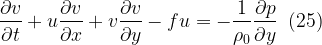
The second term of the right-hand side yields

$\displaystyle \oint{{\mathbf{u}\cdot d\left( {\frac{{d\mathbf{l}}}{{dt}}} \right)}}=\oint{{\mathbf{u}\cdot d\mathbf{u}}}=\frac{1}{2}\oint{{d\left( {\mathbf{u}\cdot \mathbf{u}} \right)}}=\frac{1}{2}\oint{{d{{{\left| \mathbf{u} \right|}}^{2}}}}=0\,\,\,(12)$

so that

$\displaystyle \frac{{dC}}{{dt}}=\oint{{\frac{{d\mathbf{u}}}{{dt}}\cdot d\mathbf{l}}}+0=\oint{{\frac{{d\mathbf{u}}}{{dt}}\cdot d\mathbf{u}}}\,\,\,(13)$

Now, refer to the Navier-Stokes equation for inviscid flow in an inertial reference frame,

$\displaystyle \frac{{d\mathbf{u}}}{{dt}}=-\frac{1}{\rho }\nabla p+\nabla \Phi \,\,\,(14)$

where we have replaced the acceleration due to gravity, g, with the potential $\displaystyle \Phi$ . Taking a scalar product of (14) and dl, and integrating along the closed contour, we get

$\displaystyle \oint{{\frac{{d\mathbf{u}}}{{dt}}\cdot d\mathbf{l}}}=\oint{{\left( {-\frac{1}{\rho }\nabla p+\nabla \Phi } \right)\cdot d\mathbf{l}}}=\int_{S}{{\left[ {\frac{1}{{{{\rho }^{2}}}}\left( {\nabla p+\nabla \Phi } \right)} \right]\cdot d\mathbf{l}}}$

$\displaystyle \therefore \oint{{\frac{{d\mathbf{u}}}{{dt}}\cdot d\mathbf{l}}}=\int_{S}{{\left[ {\frac{1}{{{{\rho }^{2}}}}\left( {\nabla \rho +\nabla p} \right)\cdot \mathbf{n}dS} \right]}}\,\,\,(15)$

where S is the surface enclosed by the closed contour and ndS is the area element normal vector. In the process of obtaining (15) use is made of Stokes’ theorem and the vector identity

$\displaystyle \nabla \times \nabla \Phi =0\,\,\,(16)$

Combining (14), (15), and (16) brings to

$\displaystyle \frac{{dC}}{{dt}}=\int_{S}{{\frac{1}{{{{\rho }^{2}}}}\left( {\nabla \rho \times \nabla p} \right)\cdot \mathbf{n}dS}}\,\,\,(17)$

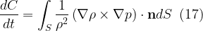
Equation (17) is a statement of Kelvin’s circulation theorem. Note that the integrand on the right-hand side is actually the solenoid term that appears in the vorticity equation. For a barotropic fluid whose density is a function only of pressure, the solenoid term is zero and circulation is conserved as fluid motion progresses. Kelvin’s circulation theorem is the fluid analog of angular momentum conservation in solid-body mechanics.

Conservation of circulation has important implications for flow on a rotating, spherical planet. If we define relative circulation over some material loop as

$\displaystyle {{C}_{r}}\equiv \oint{{{{\mathbf{u}}_{r}}\cdot d\mathbf{l}}}\,\,\,(18)$

where u_r is related to the absolute velocity vector u_aand the rotational frequency $\displaystyle \mathbf{\Omega }$ by the simple relation

$\displaystyle {{\mathbf{u}}_{r}}={{\mathbf{u}}_{a}}-\mathbf{\Omega }\times \mathbf{r}\,\,\,(19)$

We proceed to apply Stokes’ theorem to (18), giving

$\displaystyle {{C}_{r}}={{C}_{a}}-\int{{2\mathbf{\Omega }\cdot d\mathbf{A}}}={{C}_{a}}-2\Omega {{A}_{\bot }}\,\,\,(20)$

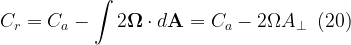
where C_a is the total or absolute circulation and $\displaystyle {{A}_{\bot }}$ is the area enclosed by the projection of the material circuit onto the plane normal to the rotation vector; that is, onto the equatorial plane (Figure 2). If the solenoidal term is zero, conservation of circulation can be stated as

$\displaystyle \frac{D}{{Dt}}\left( {{{C}_{r}}+2\Omega {{A}_{\bot }}} \right)=0\,\,\,(21)$

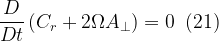
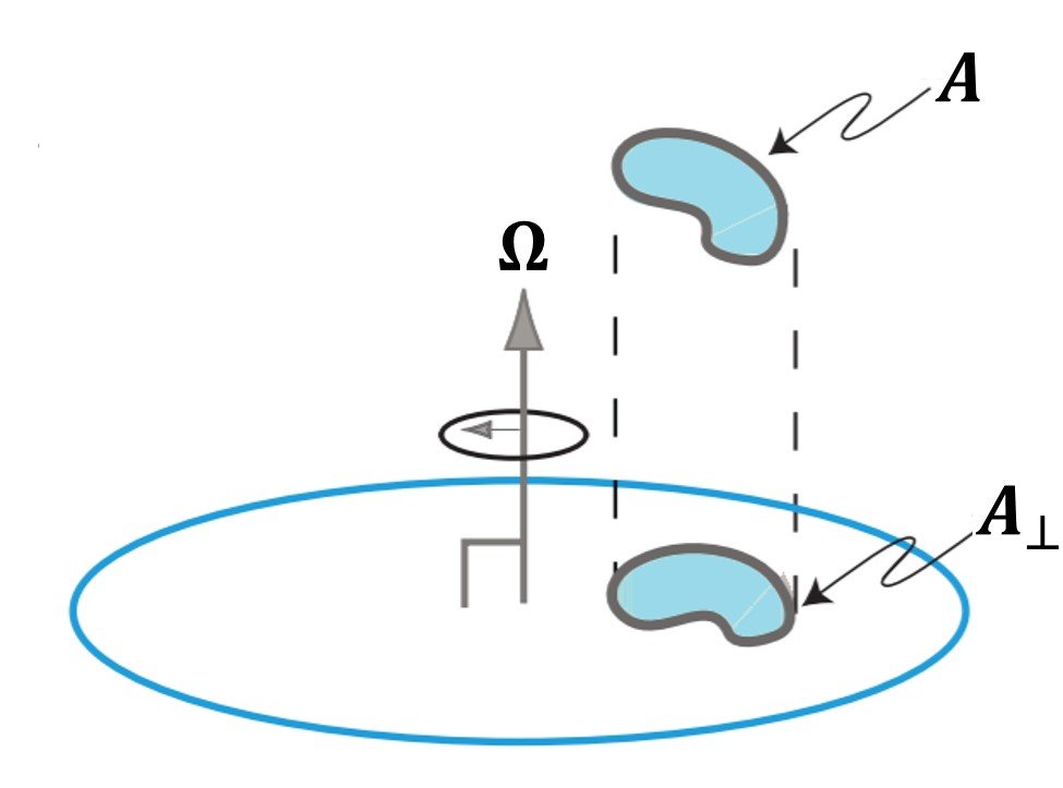
It follows that the relative circulation around a circuit changes if the orientation of the plane changes; that is, if the area of the projection onto the equatorial plane changes. In large-scale planetary flows, changes in the projected area are generally attributable to changes in latitude. Following Vallis (2017), consider the flow of a two-dimensional, infinitesimal, horizontal (i.e., tangent to the radial vector), constant-density fluid parcel at a latitude $\displaystyle \phi$ with area A, so that the projection of its area onto the equatorial plane is $\displaystyle {{A}_{\bot }}$ = $\displaystyle A\sin \phi$ and C_r = $\displaystyle {{\zeta }_{r}}$ A. If the fluid surface moves, but remains horizontal, its area is preserved (because it is incompressible) and directly from (21) its relative vorticity changes as

$\displaystyle \frac{{D{{\zeta }_{r}}}}{{Dt}}=-\frac{{2\Omega }}{A}\frac{{D{{A}_{\bot }}}}{{Dt}}=-2\Omega \frac{D}{{Dt}}\sin \phi =-{{v}_{r}}\frac{{2\Omega \cos \phi }}{a}=-\beta {{v}_{r}}\,\,\,(22)$

where

$\displaystyle \beta \equiv \frac{{df}}{{dy}}=\frac{{2\Omega \cos \phi }}{a}\,\,\,(23)$

with a being the radius. The changes in a parcel’s relative vorticity as an effect of latitudinal displacement is known as the beta-effect. It is a manifestation of the tilting term in the vorticity equation (second term in the right-hand side of (7)), and it is often the most important means by which relative vorticity does change in large-scale flow (Vallis, 2017).

Figure 2. Projection of a material circuit onto the equatorial plane.

Example 1 (Holton, 1992)

A cylindrical column of air at 30^oN with radius 100 km expands to twice its original radius. If the air is initially at rest, what is the mean tangential velocity at the perimeter after expansion?

Assuming circulation is conserved, equation (21) enables us to write

$\displaystyle {{C}_{r}}+2\Omega \sin \phi A=\text{Constant}$

Denoting initial conditions (i.e., the cylindrical column before expansion) by a subscript 0, and final conditions (i.e., the cylindrical column after expansion) by a subscript 1, we find that

$\displaystyle {{C}_{0}}+2\Omega \sin \phi {{A}_{0}}={{C}_{1}}+2\Omega \sin \phi {{A}_{1}}$

$\displaystyle \therefore {{C}_{1}}=2\Omega \sin \phi \left( {{{A}_{0}}-{{A}_{1}}} \right)+{{C}_{0}}$

Since the fluid is initially at rest, C₀ = 0. Also, $\displaystyle {{A}_{0}}$ = $\displaystyle \pi r_{0}^{2}$ and $\displaystyle {{A}_{1}}$ = $\displaystyle \pi$ $\displaystyle \times$ (2 $\displaystyle {{r}_{0}}$ )² = 4 $\displaystyle \pi r_{0}^{2}$ , because r₁ = 2r₀. Substituting above brings to

$\displaystyle \therefore {{C}_{1}}=2\Omega \sin \phi \left( {\pi r_{0}^{2}-4\pi r_{0}^{2}} \right)=2\Omega \sin \phi \left( {-3\pi r_{0}^{2}} \right)$

$\displaystyle \therefore {{C}_{1}}=2\times \left( {7.3\times {{{10}}^{{-5}}}} \right)\times \sin 30{}^\text{o}\times \left[ {-3\pi \times {{{\left( {100\times {{{10}}^{3}}} \right)}}^{2}}} \right]=-6.88\times {{10}^{6}}\,{{\text{m}}^{2}}{{\text{s}}^{{-1}}}$

Now, the tangential velocity at the perimeter after expansion can be obtained by dividing the circulation by the perimeter 2 $\displaystyle \pi$ r₁, that is,

$\displaystyle {{V}_{1}}=\frac{{{{C}_{1}}}}{{2\pi {{r}_{1}}}}=\frac{{-4.59\times {{{10}}^{6}}}}{{2\pi \times \left( {200\times {{{10}}^{3}}} \right)}}=-5.48\,\text{m/s}\leftarrow$

After expansion, the velocity at the perimeter will be close to 20 kilometers per hour. The negative sign indicates that motion is anticyclonic.

4. Potential vorticity

The x- and y-momentum equations for barotropic flows are, respectively,

$\displaystyle \frac{{\partial u}}{{\partial t}}+u\frac{{\partial u}}{{\partial x}}+v\frac{{\partial u}}{{\partial y}}-fv=-\frac{1}{{{{\rho }_{0}}}}\frac{{\partial p}}{{\partial x}}\,\,\,(24)$

$\displaystyle \frac{{\partial v}}{{\partial t}}+u\frac{{\partial v}}{{\partial x}}+v\frac{{\partial v}}{{\partial y}}-fu=-\frac{1}{{{{\rho }_{0}}}}\frac{{\partial p}}{{\partial y}}\,\,\,(25)$

Subtracting the y-derivative of equation (24) from the x-derivative of (25) and manipulating, we obtain

$\displaystyle \frac{D}{{Dt}}\left( {f+\frac{{\partial v}}{{\partial x}}-\frac{{\partial u}}{{\partial y}}} \right)+\left( {\frac{{\partial u}}{{\partial x}}+\frac{{\partial v}}{{\partial y}}} \right)\left( {f+\frac{{\partial v}}{{\partial x}}-\frac{{\partial u}}{{\partial y}}} \right)=0\,\,\,(26)$

Note that

$\displaystyle f+\frac{{\partial v}}{{\partial x}}-\frac{{\partial u}}{{\partial y}}=f+\zeta \,\,\,(27)$

represents the sum of ambient vorticity (f) and relative vorticity ( $\displaystyle \zeta$ = $\displaystyle \partial v$ / $\displaystyle \partial x$ – $\displaystyle \partial u$ / $\displaystyle \partial y$ , where we have dropped the subscript r for brevity). We also need the continuity equation, which for a geostrophic flow reads

$\displaystyle \frac{{\partial h}}{{\partial t}}+\frac{\partial }{{\partial x}}\left( {hu} \right)+\frac{\partial }{{\partial y}}\left( {hv} \right)=0\,\,\,(28)$

and can be restated as

$\displaystyle \frac{{Dh}}{{Dt}}+\left( {\frac{{\partial u}}{{\partial x}}+\frac{{\partial v}}{{\partial y}}} \right)h=0\,\,\,(29)$

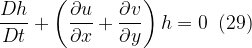
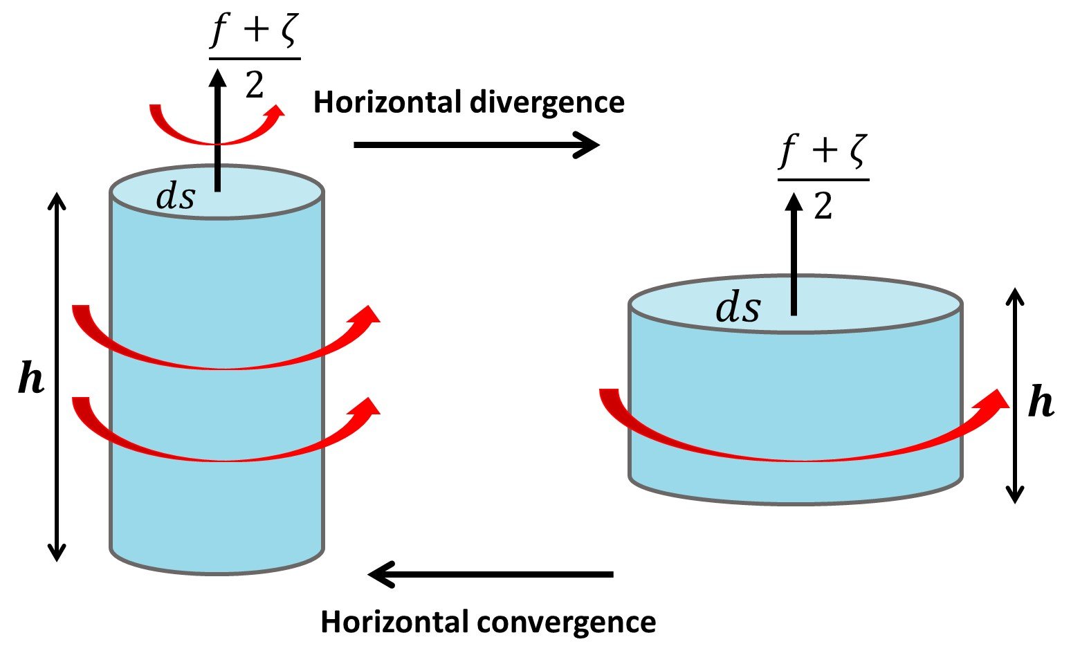
At this point, we consider a narrow fluid column of horizontal cross-section ds and height h, giving a volume hds. In view of conservation of volume in an incompressible fluid, we may write

$\displaystyle \frac{d}{{dt}}\left( {hds} \right)=0\,\,\,(30)$

This is a simple geometrical constraint on the volume of the fluid column which, if squeezed vertically (decreasing h), must stretch horizontally (increasing ds), and vice versa (Figure 3).

Figure 3. Conservation of volume in a fluid column.

Combining (30) with the modified continuity equation gives an equation for the rate of change of the element cross-section ds:

$\displaystyle \frac{D}{{Dt}}\left( {ds} \right)=\left( {\frac{{\partial u}}{{\partial x}}+\frac{{\partial v}}{{\partial y}}} \right)ds\,\,\,(31)$

This equation indicates that horizontal divergence ( $\displaystyle \partial u$ / $\displaystyle \partial x$ + $\displaystyle \partial v$ / $\displaystyle \partial y$ > 0) is accompanied by widening of the cross-sectional area ds, whereas convergence ( $\displaystyle \partial u$ / $\displaystyle \partial x$ + $\displaystyle \partial v$ / $\displaystyle \partial y$ < 0) causes a narrowing of the cross-section. Now, introducing (26) into (30) yields

$\displaystyle \frac{d}{{dt}}\left[ {\left( {f+\zeta } \right)ds} \right]=0\,\,\,(32)$

This result implies that the product (f + $\displaystyle \zeta$ )ds is conserved by the fluid parcel. As the reader will surely notice, this is a product of vorticity and cross-sectional area, and hence constitutes a measure of circulation. Thus, (32) indicates that circulation is conserved in the rotating, two-dimensional flow at hand.

If both circulation and volume are conserved, so is their ratio. This ratio is useful because it does away with the cross-section of the fluid parcel and depends only on local variables of the flow field,

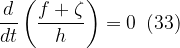
$\displaystyle \frac{d}{{dt}}\left( {\frac{{f+\zeta }}{h}} \right)=0\,\,\,(33)$

where

$\displaystyle q=\frac{{f+\zeta }}{h}=\frac{{f+{{\partial v}}/{{\partial x}}\;-{{\partial u}}/{{\partial y}}\;}}{h}\,\,\,(34)$

is called the potential vorticity. The preceding analysis interprets potential vorticity as circulation per volume. The conservation of potential vorticity was first introduced by Rossby and then in a more general form by Ertel, and plays a crucial role in geophysical flows.

For example, conservation of potential vorticity enables clever ways to reproduce large-scale flows in laboratory settings. Consider potential-vorticity conservation in a large-scale geophysical vortex, atmospheric or oceanic in nature, with a constant depth H₀. When this vortex is shifted northwards, f increases in order to keep (f + $\displaystyle \zeta$ )/H₀ constant. Per the beta-effect, a cyclonic vortex ( $\displaystyle \zeta$ > 0) moving northwards becomes weaker, while an anticyclonic vortex ( $\displaystyle \zeta$ < 0) will intensify when moving northwards. Conservation of potential vorticity can be exploited to model the planetary $\displaystyle \beta$ -effect in a rotating tank by a suitably chosen bottom topography. Changes of the Coriolis parameter f with the northward coordinate y, as in the $\displaystyle \beta$ -plane approximation f(y) = f₀ + $\displaystyle \beta$ y, can be dynamically mimicked in the laboratory by a variation in the water depth H(y), according to

$\displaystyle \frac{{f\left( y \right)+\zeta }}{{{{H}_{0}}}}=\frac{{{{f}_{0}}+\zeta }}{{H\left( y \right)}}=\text{Constant}\,\,\,\text{(35)}$

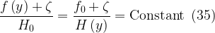
with H₀ denoting the constant fluid depth in the geophysical case (leftmost part of the equation) and f₀ = 2 $\displaystyle \Omega$ denoting the constant Coriolis parameter in the rotating tank experiment (middle part of the equation). For small Rossby number Ro values and weak topography effects, the $\displaystyle \beta$ -plane approximation f(y) = f₀ + $\displaystyle \beta$ y can be straightforwardly modelled by a uniformly sloping bottom in a rotating-fluid tank. This configuration is commonly known as a ‘topographic $\displaystyle \beta$ -plane.’ For details, see van Heijst (2010) and references therein.

Let’s close this post with another solved example.

Example 2 (Holton, 1992)

An air column at 60^oN with relative vorticity $\displaystyle \zeta$ = 0 initially stretches from the surface to a fixed tropopause at 10-km height. If the air column moves until it is over a mountain barrier 2.5 km high at 45^oN, what is its relative vorticity as it passes the mountaintop?

Denoting initial and final conditions by subscripts 0 and 1, respectively, we can state the conservation of potential vorticity as

$\displaystyle \frac{{{{\zeta }_{0}}+{{f}_{0}}}}{{{{H}_{0}}}}=\frac{{{{\zeta }_{1}}+{{f}_{1}}}}{{{{H}_{1}}}}=\text{Constant}$

Noting that $\displaystyle {{\zeta }_{0}}$ = 0 because the column is initially at rest and solving for $\displaystyle {{\zeta }_{1}}$ + f₁,

$\displaystyle {{\zeta }_{1}}+{{f}_{1}}=\frac{{{{H}_{1}}}}{{{{H}_{0}}}}\times {{f}_{0}}=\frac{{{{H}_{1}}}}{{{{H}_{0}}}}\times 2\Omega \sin {{\phi }_{0}}$

$\displaystyle {{\zeta }_{1}}+{{f}_{1}}=\frac{{{{H}_{1}}}}{{{{H}_{0}}}}\times 2\Omega \sin {{\phi }_{0}}=\frac{{7.5}}{{10}}\times 2\times \left( {7.3\times {{{10}}^{{-5}}}} \right)\times \sin 60{}^\text{o}=9.48\times {{10}^{{-5}}}\,{{\text{s}}^{{-1}}}$

But, as the air column reaches 45^oN latitude,

$\displaystyle {{f}_{1}}=2\Omega \sin {{\phi }_{1}}=2\times \left( {7.3\times {{{10}}^{{-5}}}} \right)\times \sin 45{}^\text{o}=1.03\times {{10}^{{-4}}}\,{{\text{s}}^{{-1}}}$

so that

$\displaystyle {{\zeta }_{1}}=9.48\times {{10}^{{-5}}}-1.03\times {{10}^{{-4}}}=-8.20\times {{10}^{{=6}}}\,{{\text{s}}^{{-1}}}\leftarrow$

The negative sign indicates that motion becomes anticyclonic as the air column reaches the mountaintop.

References

• CUSHMAN-ROISIN, B. and BECKERS, J.-M. (1993). Introduction to Geophysical Fluid Dynamics. Boston: Academic Press.

• HOLTON, J.R. (1992). An Introduction to Dynamic Meteorology. 3rd edition. Boston: Academic Press.

• ÖSZOY, E. (2020). Geophysical Fluid Dynamics I. Berlin/Heidelberg: Springer.

• PEDLOSKY, J. (1987). Geophysical Fluid Dynamics. 2nd edition. Berlin/Heidelberg: Springer.

• VALLIS, G.K. (2017). Atmospheric and Oceanic Fluid Dynamics. 2nd edition. Cambridge: Cambridge University Press.

• Van Heijst, G.J.F. (2010). Dynamics of vortices in rotating and stratified fluids. In: FLÓR, J.-B. (Ed.). Fronts, Waves and Vortices in Geophysical Flows. Berlin/Heidelberg: Springer.

Vorticity, Circulation, and Potential Vorticity

Subscribe to our Mailing List!

Featured Posts

A Primer on NAND Flash Memories

Solidification Time and Chvorinov’s Rule

Step-Growth Polymerization, the Carothers Equation, and the Flory-Schulz Distribution

More Articles

Glacier Profiles: The Parabolic, Vialov, and Bueler Models

Bagnold’s Blown Sand Transport and Saltation

Fields of Study

More

© 2024 Montogue Quiz

Subscribe to
our Mailing List!

Subscribe to our Mailing List!

Subscribe to receive our latest materials in your inbox.

Homework Help

© 2024 Montogue Quiz

Subscribe to our Mailing List!