Electrokinetics and Electroosmotic Flow

Electroosmosis has been a known phenomenon since the 19th century, but it wasn’t until recent decades, with the advent of microfluidic technology and immense progress in colloid science, that it became a common research topic. In this post, I provide a rundown of several aspects of electroosmotic flow theory.

1. Zeta potential and the electric double layer

Most substances acquire a surface electric charge when brought into contact with an aqueous (polar) medium. The effect of any charged surface in an electrolyte solution is to influence the distribution of nearby ions in the solution. Ions of opposite charge to that of the surface, known as counterions, are attracted toward the surface, while ions of like charges, known as co-ions, are repelled from the surface. These attraction and repulsion phenomena, when combined with the mixing tendency resulting from the random thermal motion of the ions, leads to the formation of a so-called electrical double layer, or EDL for short. The electric double layer is a region close to the charged surface in which there is an excess of counterions over coions (Panigrahi, 2016).

Because of the electrostatic interaction, the counterion concentration near the solid surface is higher than that in the bulk fluid away from the solid surface. Immediately next to the solid surface, there is a layer of ions that are strongly attracted to the solid surface and are immobile. This layer, known as the compact or Stern layer, is normally less than 1 nm thick. From the compact layer to the uniform bulk liquid, the counterion concentration gradually reduces to that of the neutral running fluid. Ions in this region are affected less by the electrostatic interaction and are mobile. This layer is called the diffuse or Gouy-Chapman layer of the EDL. The thickness of the diffuse layer depends on the bulk ionic concentration and electrical properties of the liquid, ranging from a few nanometers for high ionic concentration solutions up to several micrometers for distilled water and pure organic liquids. The boundary between the compact layer and the diffuse layer is usually referred to as the shear plane. The shear plane itself is somewhat arbitrary but can be defined as the plane at which the mobile portion of the diffuse layer can “slip” or flow past the charged surface (Probstein, 1994). The electrical potential at the solid-liquid surface is difficult to measure directly; on the other hand, the electrical potential at the shear plane can be measured experimentally; it is called the zeta potential.

The concentration of ions in the diffuse region of the EDL decays roughly exponentially as it approaches the bulk fluid; the thickness of the diffuse region is of the order of the so-called Debye length $\displaystyle {{\lambda }_{D}}$ , a parameter given by

$\displaystyle {{\lambda }_{D}}={{\left( {\frac{{\varepsilon {{k}_{b}}T}}{{2{{z}^{2}}{{e}^{2}}{{c}_{0}}}}} \right)}^{{{1}/{2}\;}}}\,\,\,(1)$

where $\displaystyle \varepsilon$ is the permittivity of the medium (i.e., $\displaystyle {{\varepsilon }_{r}}$ $\displaystyle \times$ $\displaystyle {{\varepsilon }_{0}}$ ), where $\displaystyle {{\varepsilon }_{r}}$ is the relative permittivity and $\displaystyle {{\varepsilon }_{0}}$ = 8.85 $\displaystyle \times$ 10^-12 F/m is the vacuum permittivity), k_b $\displaystyle \approx$ 1.38 $\displaystyle \times$ 10^-23 J/K is Boltzmann’s constant, T is temperature, z is ionic valence, e $\displaystyle \approx$ 1.60 $\displaystyle \times$ 10^-19 C is the elemental charge, and c₀ is the electrolyte concentration. The Debye length is the reciprocal square root of the Debye-Hückel parameter $\displaystyle \kappa$ = $\displaystyle \lambda _{{\acute{\ }D}}^{{-2}}$ , which will appear in some of the upcoming equations. For an aqueous solution of a symmetric electrolyte at 25^oC, the Debye length can be estimated as

$\displaystyle {{\lambda }_{D}}=9.61\times {{10}^{{-9}}}{{\left( {{{z}^{2}}c} \right)}^{{-{1}/{2}\;}}}\,\,\,(2)$

where $\displaystyle {{\lambda }_{D}}$ is in meters, z is the ionic valence, and c is the concentration in mol/m³. For an univalent electrolyte at 1 mol/m³, $\displaystyle {{\lambda }_{D}}$ $\displaystyle \approx$ 9.6 nm; for an univalent electrolyte at 100 mol/m³, $\displaystyle {{\lambda }_{D}}$ $\displaystyle \approx$ 0.96 nm.

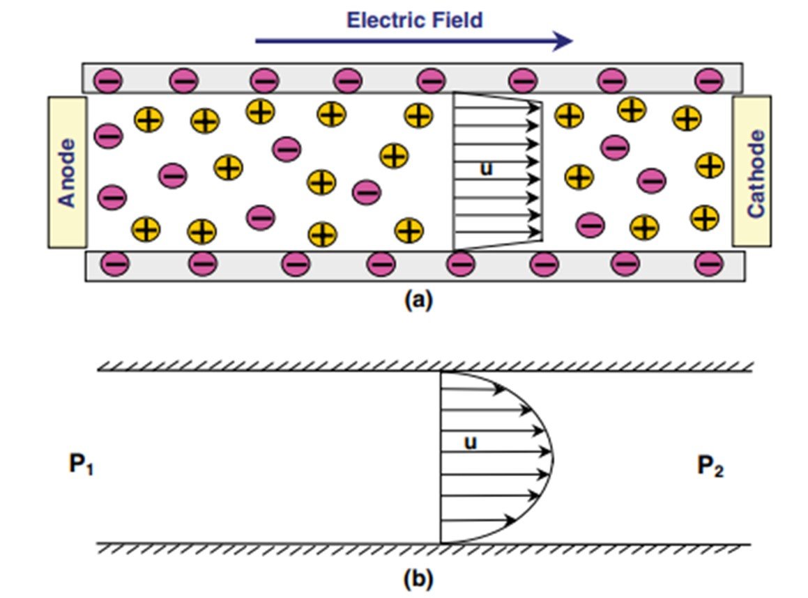
Electroosmotic flow is the bulk liquid motion that results when an externally applied electric field interacts with the net surplus of charged ions in the diffuse part of an electrical double layer. EO flow is one of the four kinds of electrokinetic phenomena; the others are electrophoresis, streaming potential, and sedimentation potential. EO flow has recently become an attractive research topic for microfluidics and ‘lab-on-a-chip’ applications. Erickson (2015) mentions some of the factors that have contributed to the growing interest in electroosmosis. The most important such factor has to do with the flat velocity profile observed in a parallel-plate electroosmosis, which, in contrast to the parabolic profile displayed in Poiseuille flow (see Figure 1), allows for minimal dispersion and is less disrupted by localized variations in viscosity. What’s more, electroosmotic flow is a surface-driven phenomenon, so electroosmotic velocity is largely independent of channel size. Lastly, electroosmotic flow offers an additional advantage when dealing with interconnected or branching channels, as flow in these can be controlled by switching voltage direction, with no need for valves or other moving parts.

One important disadvantage of electroosmotic flows is that they are characterized by high electric field requirements (>100 V/cm) and low flow speeds (<1 mm/s); of course, speeds can be readily increased by subjecting the system to a stronger electric field, but more intense electric fields are often accompanied by Joule heating, sometimes to the point of causing localized changes in viscosity and even in-channel boiling. Electroosmotic flows are also highly sensitive to surface contamination.

Figure 1. Comparison between velocity profiles for (a) electroosmotic and (b) pressure-driven flows.

2. The Helmholtz-Smoluchowski equation

As in so many fluid flow problems, we start our analysis of EO flow with a form of the momentum (Navier-Stokes) equation:

$\displaystyle \rho \frac{{D\mathbf{u}}}{{Dt}}=\nabla \cdot \mathbf{T}+\rho g+{{\rho }_{E}}\mathbf{E}\,\,\,(3)$

where $\displaystyle \rho$ is fluid density, u is the velocity vector, D()/Dt denotes a material derivative, T is the stress tensor, g $\displaystyle \approx$ 9.81 m/s², $\displaystyle {{\rho }_{E}}$ is the electric charge density, and E is the electric field vector. Neglecting gravitational forces and supposing the flow to be an inertia-free capillary flow, with no pressure gradient, equation (3) reduces to a balance between viscous and electrical forces:

$\displaystyle \mu {{\nabla }^{2}}\mathbf{u}=-{{\rho }_{E}}\mathbf{E}\,\,\,(4)$

with x as the coordinate directed along the axis toward the cathode and u the velocity component in that direction, we surmise that, for a long capillary, the derivatives of u with respect to the longitudinal direction x are zero and u is a function of the transverse coordinate y only. If, moreover, the diffuse layer thickness $\displaystyle {{\lambda }_{D}}$ is small compared with the channel dimension a, then the curvature terms can be neglected and equation (4) reduces to the one-dimensional form pertaining to a long plane channel or an infinite plane surface:

$\displaystyle \mu \frac{{{{\partial }^{2}}u}}{{\partial {{y}^{2}}}}=-{{\rho }_{E}}{{E}_{x}}\,\,\,(5)$

But, replacing $\displaystyle {{\rho }_{E}}$ with Poisson’s equation, that is,

$\displaystyle {{\nabla }^{2}}\phi =-\frac{{{{\rho }_{E}}}}{\varepsilon }\,\,\,(6)$

we get

$\displaystyle \mu \frac{{{{\partial }^{2}}u}}{{\partial {{y}^{2}}}}=\varepsilon \frac{{{{\partial }^{2}}\phi }}{{\partial {{y}^{2}}}}{{E}_{{_{x}}}}\,\,\,(7)$

The component E_x of the electric field is parallel to the surface in the positive x-direction. Integrating (7) once brings to

$\displaystyle \mu \frac{{\partial u}}{{\partial y}}=\varepsilon \frac{{\partial \phi }}{{\partial y}}{{E}_{{_{x}}}}\,\,\,(8)$

where at the edge of the diffuse layer (y $\displaystyle \to$ $\displaystyle \infty$ ) we have set $\displaystyle \partial$ u/ $\displaystyle \partial$ y = $\displaystyle \partial$ $\displaystyle \phi$ / $\displaystyle \partial$ y = 0. Integrating a second time and setting $\displaystyle \phi$ = $\displaystyle \zeta$ (the zeta potential) at u = 0, we find

$\displaystyle U=-\frac{{\varepsilon \zeta {{E}_{x}}}}{\mu }\,\,\,(9)$

This formula for the electroosmotic velocity past a plane charged surface is sometimes known as the Helmholtz-Smoluchowski equation. It shows that the electroosmotic flow velocity is linearly proportional to the applied electrical field strength and the zeta potential. The negative sign indicates the flow direction and has to do with the sign of $\displaystyle \zeta$ : if the zeta potential is negative (i.e., the wall surface is negatively charged), the excess counterions in the diffuse layer are positive, therefore the electroosmotic flow in the microchannel is towards the negative electrode. It is commonplace to condense the factor $\displaystyle \varepsilon \zeta$ / $\displaystyle \mu$ in a single parameter $\displaystyle {{\mu }_{E}}$ , known as the electroosmotic mobility, so that

$\displaystyle \left| U \right|={{\mu }_{E}}{{E}_{x}}\,\,\,(10)$

3. The Poisson-Boltzmann equation and elementary solutions

In order to characterize an electrokinetic flow, we must be able to describe its potential distribution. The equation to use is the Poisson equation, which we’ve already stated in (6) but repeat here for convenience:

$\displaystyle {{\nabla }^{2}}\phi =-\frac{{{{\rho }_{E}}}}{\varepsilon }\,\,\,(6)$

Assuming the equilibrium Boltzmann distribution to be applicable, the number concentration of type-i ion in a symmetric electrolyte solution has the form

$\displaystyle {{n}_{i}}={{n}_{{i\infty }}}\exp \left( {-\frac{{{{z}_{i}}e\phi }}{{{{k}_{b}}T}}} \right)\,\,\,(11)$

where $\displaystyle {{n}_{{i\infty }}}$ and z_i are the bulk ionic concentration and the valence of type-i ions, respectively, and other variables have the same meaning as in equation (1). The net volume charge density $\displaystyle {{\rho }_{E}}$ is proportional to the concentration difference between symmetric cations and anions, so that

$\displaystyle {{\rho }_{E}}=ze\left( {{{n}_{+}}-{{n}_{-}}} \right)=-2ze{{n}_{\infty }}\sinh \left( {\frac{{ze\phi }}{{{{k}_{b}}T}}} \right)\,\,\,(12)$

Substituting $\displaystyle {{\rho }_{E}}$ into (6) yields

$\displaystyle {{\nabla }^{2}}\phi =\frac{{2ze{{n}_{\infty }}}}{\varepsilon }\sinh \left( {\frac{{ze\phi }}{{{{k}_{b}}T}}} \right)\,\,\,(13)$

At this point, we define the Debye-Hückel parameter

$\displaystyle {{\kappa }^{2}}\equiv \frac{{2{{z}^{2}}{{e}^{2}}{{n}_{\infty }}}}{{\varepsilon {{k}_{b}}T}}\,\,\,(14)$

Then, we introduce the dimensionless electrical potential

$\displaystyle \Phi =\frac{{ze\phi }}{{{{k}_{b}}T}}\,\,\,(15)$

so that (13) can be restated as

$\displaystyle {{\nabla }^{2}}\Phi ={{\kappa }^{2}}\sinh \left( \Phi \right)\,\,\,(16)$

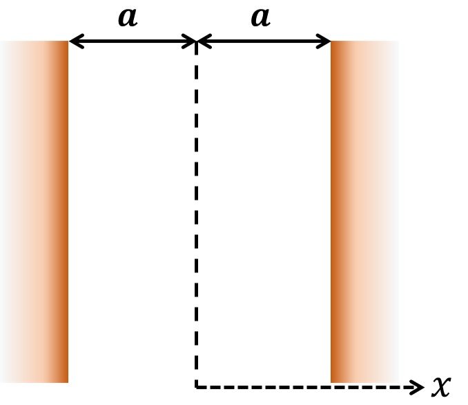
This relationship is known as the Poisson-Boltzmann equation. Upon solving this equation with the appropriate boundary conditions, the electrical potential distribution $\displaystyle \phi$ of the EDL can be established, and thence the charge density distribution $\displaystyle {{\rho }_{E}}$ .

We now proceed to obtain a simple solution for the electric double layer. With reference to Figure 2, we set the origin of the x-axis in the middle plane between the two plates, so the P-B equation can be restated as

$\displaystyle \frac{{{{d}^{2}}\Phi }}{{d{{{\bar{X}}}^{2}}}}=K\sinh \left( \Phi \right)\,\,\,(17)$

where $\displaystyle \bar{X}$ = x/a, K = $\displaystyle \kappa$ a, and $\displaystyle \kappa$ is the Debye-Hückel parameter. If the distance a is much larger than the EDL thickness, the boundary conditions are:

$\displaystyle \bar{X}=0\,\,\,;\,\,\,\Psi =0\,\,\,(18.1)$

which means that the potential infinitely away from the surface is zero; and

$\displaystyle \bar{X}=1\,\,\,;\,\,\,\Phi =\frac{{ze\zeta }}{{{{k}_{b}}T}}\,\,\,(18.2)$

which is the dimensionless potential at the shear plane. Once the BCs have been posed, we note that, if the electrical potential ze $\displaystyle \phi$ is small compared to the thermal energy k_bT of the ions, the P-B equation can be linearized to

$\displaystyle \frac{{{{d}^{2}}\Phi }}{{d{{{\bar{X}}}^{2}}}}={{K}^{2}}\Phi \,\,\,(19)$

This shortcut to a simpler equation is known as the Debye-Hückel approximation. The solution to (19) is readily found to be

$\displaystyle \Phi \left( {\bar{X}} \right)=\frac{{ze\zeta }}{{{{k}_{b}}T\sinh \left( K \right)}}\left| {\sinh \left( {K\bar{X}} \right)} \right|\,\,\,(20)$

Figure 2. Two identical flat surfaces.

Another noteworthy solution arises if we consider a flat surface in contact with an infinitely large aqueous medium. Setting the origin of the coordinate system on the wall, as illustrated in Figure 3, the P-B equation in dimensional form is expressed as

$\displaystyle \frac{{{{\partial }^{2}}\phi }}{{\partial {{x}^{2}}}}=\frac{{2ze{{n}_{\infty }}}}{\varepsilon }\sinh \left( {\frac{{ze\phi }}{{{{k}_{b}}T}}} \right)\,\,\,(21)$

The boundary conditions are

$\displaystyle x=0\,\,\,;\,\,\,\phi ={{\phi }_{0}}\approx \zeta \,\,\,(22.1)$

That is, the potential at the surface or shear plane is close to the zeta potential; and

$\displaystyle x=\infty \,\,\,;\,\,\,\phi =0\,\,\,(22.2)$

That is, the potential infinitely away from the surface equals zero. Using the Debye-Hückel approximation, the potential distribution is found to be

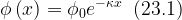
$\displaystyle \phi \left( x \right)={{\phi }_{0}}{{e}^{{-\kappa x}}}\,\,\,(23.1)$

or, equivalently,

$\displaystyle \phi \left( x \right)\approx \zeta {{e}^{{-\kappa x}}}\,\,\,(23.2)$

The dimensionless factor $\displaystyle \kappa$ x is sometimes known as the electrokinetic distance, and serves as a measure of the distance relative to the EDL thickness.

We close by noting that there exists an analytical solution for the ‘full’ P-B equation (21) as applied to the flat-surface system (Fig. 3). The solution is

$\displaystyle \phi \left( x \right)=\frac{{2{{k}_{b}}T}}{{ze}}\ln \left[ {\frac{{1+\exp \left( {-\kappa x} \right)\tanh \left( {{{ze\zeta }}/{{4{{k}_{b}}T}}\;} \right)}}{{1-\exp \left( {-\kappa x} \right)\tanh \left( {{{ze\zeta }}/{{4{{k}_{b}}T}}\;} \right)}}} \right]\,\,\,(24)$

Figure 3. Flat surface in an infinitely large liquid.

4. Entry length in electroosmotic flow

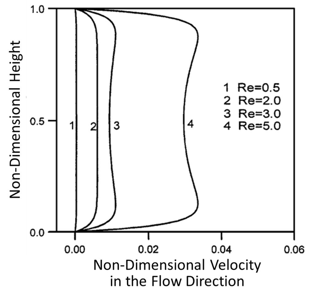
Yang et al. (2001) assessed entry length phenomena in electroosmotic flows. Like so many hydrodynamic systems, a flow entering a pipe (or a microchannel, for that matter) does not immediately attain a steady motion; the flow must first cover a distance, known as the entrance length, before full hydrodynamic accommodation can take place. Yang et al. (2001) investigated entry dynamics in electroosmotic flow of a rectangular microchannel; the flow-entry velocity profiles achieved for different Reynolds numbers are shown in Figure 4. Clearly, the velocity profile achieved is markedly flat for Re = 0.5 and 2.0, as one would expect for electroosmotic flow; however, the velocity profile becomes somewhat concave for increasing Re. When the Reynolds number is small, the viscous component of flow is prevalent and fluid near the walls drags the fluid of the central channel, leading to a flat velocity profile. As the Reynolds number is made larger, however, electrokinetic forces at the walls cause the charge-rich boundaries of the channel to flow faster than the charge-poor central portion of the channel, leading to a concave velocity profile.

Figure 4. Velocity distributions for electroosmotic flow in a rectangular microchannel at various Reynolds numbers.

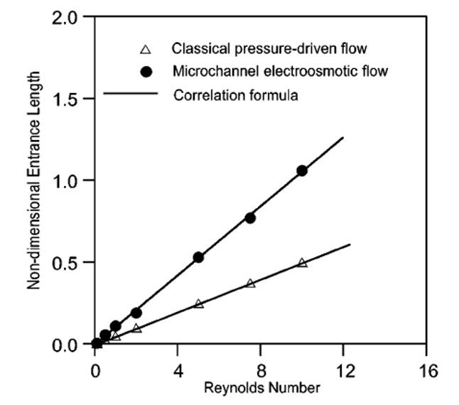
Yang et al. (2001) went on to show that, much like pressure-driven systems, electroosmotic flows can have their entrance lengths calculated on the basis of Reynolds number, as shown in Figure 5. The entry length for a classical fluid-dynamic flow is estimated as L_e $\displaystyle \approx$ 0.06Re, whereas that of an electroosmotic flow is such that L_e $\displaystyle \approx$ 0.11Re. The greater entrance length for electroosmotic flow is probably related to the fact that, in addition to viscous drag, EO flow must also overcome the attraction between fluid and electric double layer, so that a greater distance is needed before the flow becomes fully developed.

Figure 5. Nondimensional entrance length versus Reynolds number for electroosmotic and pressure-driven flows.

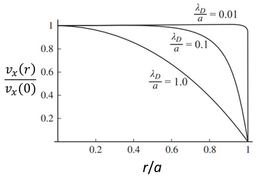
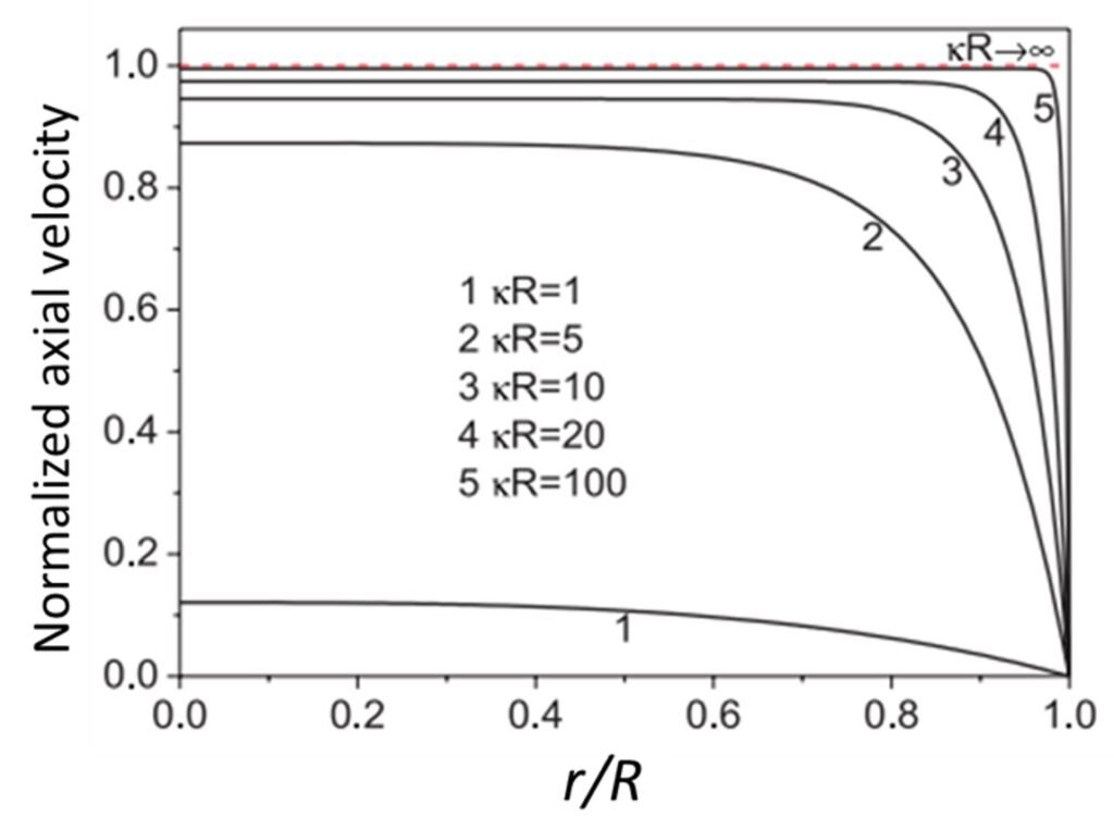
5. Debye length overlap

What happens when the Debye length $\displaystyle {{\lambda }_{D}}$ becomes comparable in size to the transverse length scale a of the channel? Figure 6 shows normalized velocity profiles for a normalized radial distance r/a in a cylindrical capillary with radius a, considering three ratios a/ $\displaystyle {{\lambda }_{D}}$ , namely 0.01, 0.1, and 1.0. Notice that for small values of $\displaystyle {{\lambda }_{D}}$ /a, a nearly flat velocity profile is observed. As $\displaystyle {{\lambda }_{D}}$ is increased, and eventually becomes comparable to the radius of the capillary, the profile changes to a paraboloid shape. Panigrahi (2016) explains this by noting that, when the Debye screening length is large compared to the transverse dimension of a channel, the screening of charges on the wall becomes incomplete, and the electrical potential does not vary much across the channel. As a result, the Debye layers reaching out from the walls overlap in the center and thereby prevent a charge-neutral bulk flow from being established. This implies that the velocity profile likewise does not vary considerably, and the no-slip boundary condition is felt strongly even at the center of the channel. The electroosmotic flow is then strongly suppressed in the limit of Debye layer overlap, that is, when $\displaystyle {{\lambda }_{D}}$ $\displaystyle \ge$ a.

Figure 6. Normalized velocity profiles for three Debye length-channel radius ratios.

6. Electroosmotic flow and non-Newtonian fluids

Since so many applications of microfluidics involve eminently nonlinear fluids, there is a rapidly growing body of research on electroosmotic flow of non-Newtonian fluids. The most important example, arguably, is human blood, which has been described as a Bingham plastic, a power-law fluid, and a Casson fluid. Of these, blood is most straightforwardly described as a power-law shear-thinning fluid, with index ranging between 0 and 1. It is noteworthy, however, that human blood can also show Bingham-plastic behavior, albeit with a very low yield stress and only when enriched with a substantial concentration of fibrinogen (Das and Chakraborty, 2006). It follows that for all practical purposes the Bingham plastic characteristics of blood can be neglected and a power-law or Casson-fluid framework suffices for practical applications. For example, Tang et al. (2009) used a lattice Boltzmann method to simulate flowing of power-law fluids in a parallel-plate configuration. Power-law fluids are mostly favored because of their simplicity in assessing a broad range of non-Newtonian fluids with a minimum of adjustment parameters.

Recalling that plug-like flow is a desirable feature in electroosmosis, Tang’s team noted that previous work had shown that a Newtonian fluid displays a plug-shaped velocity profile when the ratio of channel height to Debye length exceeds about 10. With this in mind, Tang’s team employed a combination of parameters that led to a Debye length $\displaystyle {{\lambda }_{D}}$ = 0.02915 $\displaystyle \mu$ m and studied parallel-plate flow of fluids with different power-law indices. They found that velocity profiles for Newtonian flow remained parabolic for heights H = 0.1 $\displaystyle \mu$ m and 0.2 $\displaystyle \mu$ m, but became plug-like when H = 0.4 $\displaystyle \mu$ m. In contrast, a shear-thickening fluid with index n = 1.5 did not flow in plug-like fashion until H was made as large as 1.0 $\displaystyle \mu$ m, which is more than 30 times the Debye length at hand. Lastly, a shear-thinning fluid with index n = 0.5 exhibited plug-like profiles for H as low as 0.05 $\displaystyle \mu$ m. Simply put, Tang’s team found that achieving plug-shaped electroosmotic flow with shear-thinning fluids may be easier than with shear-thickening ones.

A similar finding has been reported by Vasu and De (2010), who devised a solution for electroosmosis of power-law fluids flowing in rectangular microchannels, with no resort to the Debye-Hückel approximation. Those workers found that pseudoplastic (shear-thinning) fluids flowed with a faster and more uniform velocity profile when compared to dilatant (shear-thickening) fluids under the same thermophysical conditions. Vasu and his colleague note that this could be a boon for practical applications, since the flow index n can be manipulated (lowered) through temperature or pH, giving rise to different velocity profiles.

Berli (2009) assessed the flow rate, output pressure and thermodynamic efficiency attained when typical non-Newtonian fluids are electrokinetically pumped through single microchannels. Berli found that pumps based on non-Newtonian fluids have appreciable advantages, such as an inherent ease to achieve good pumping performances with low electric field intensities and large channel diameters. Importantly, that worker also evaluated the thermodynamic efficiency for electroosmotic pumping of power-law fluids, and found that the output pressure and pumping efficiency for shear-thinning fluids could be several times higher than those for Newtonian fluids under the same experimental conditions.

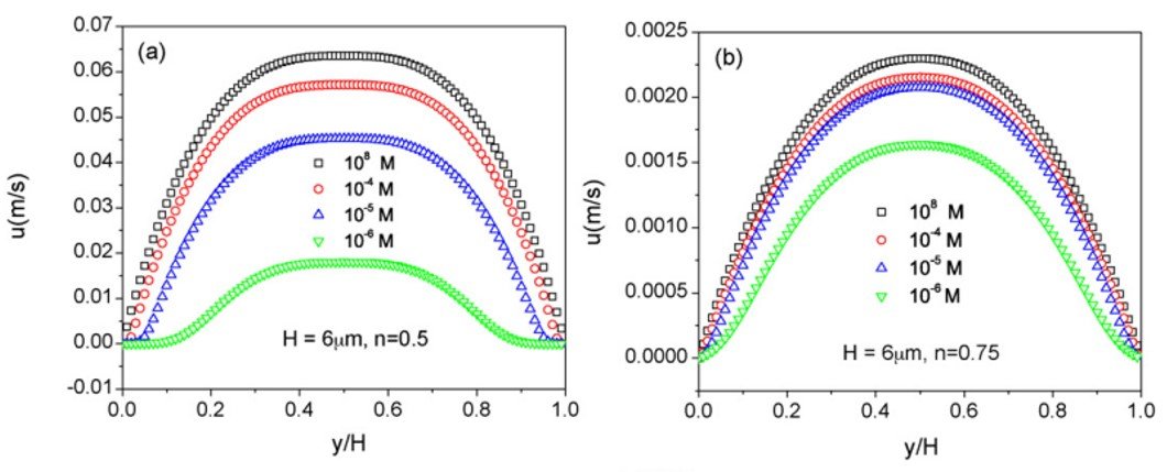
Tang et al. (2010) studied the occurrence of an electroviscous effect in power-law non-Newtonian fluids with different flow indices n, flowing in a parallel-plate channel of height H. Figure 7 shows the velocity profiles for various ionic concentrations at flow indices n = 0.5 and 0.75. Clearly, the velocity profile gets flattened and the magnitude decreases as the ionic concentration decreases; most importantly, comparison between different figures at the same concentration reveals that, for shear-thinning fluids at least, the velocity reduction associated with the electroviscous effect increases as flow index decreases.

Figure 7. Velocity profiles for microchannel flow of a power-law fluid with (a) n = 0.5 and (b) n = 0.75 at different ionic concentrations. From Tang et al. (2010).

Although most studies on non-Newtonian electroosmosis have relied on the power-law approach, some researchers have made strides with other rheological formulations. One example is Zhao and Yang (2011), who modelled electroosmotic flow for Carreau fluids, a five-parameter constitutive model that includes Newtonian and power-law behavior as special cases, with the aim of assessing effects on electroosmotic mobility. Those workers found that the electroosmotic velocity of Carreau fluids increases with surface zeta potential but decreases with power-law exponent. The relationship with the Weissenberg number (i.e., the dimensionless relaxation time constant) was a little more nuanced, in that, as Wi increased, electroosmotic mobility increased for shear-thinning fluids and decreased for shear-thickening fluids.

Zhao and Yang (2013) developed analytical solutions for electroosmotic flow of non-Newtonian power-law fluids. In contrast to studies conducted until that time, Zhao and his colleague employed a cylindrical microchannel in lieu of a parallel-plate geometry. Interestingly, they found that velocity profiles changed in accordance with variations of the factor $\displaystyle \kappa$ R, where $\displaystyle \kappa$ is the Debye-Hückel parameter and R is the radius of the microchannel (Figure 8). For small $\displaystyle \kappa$ R ( $\displaystyle \sim$ 1), the electric double layer occupies the entire channel, and the electrostatic body force is present throughout the whole channel domain; a parabolic velocity profile is observed, much like in Poiseuille flow. As $\displaystyle \kappa$ R increases substantially, however, variation of the velocity becomes increasingly restricted to the near-wall region, and the velocity acquires constant values in the central bulk region of the channel. The fact that the bulk fluid velocity may depend on radius R – that is, on the geometry of the channel – is rather striking, since, as Zhao and his colleague noted, there are no geometrical parameters in the Helmholtz-Smoluchowski velocity equation.

Figure 8. Normalized velocity profiles for different values of product $\displaystyle \kappa$ R, as predicted by Zhao and Yang (2013).

7. Electroosmotic flow and branching channels

While our discussion has focused on electroosmotic flow in single microchannels, modern microfluidic devices consist of not one but a myriad of successively branching channels. Jing and Yi (2019) tackled this issue by using a tree-like branching scheme of cylindrical microchannels in the spirit of Murray’s law. The basic branching relationship they found is

$\displaystyle R_{0}^{2}=R_{1}^{2}+R_{2}^{2}\,\,\,(25)$

where R₀ is the radius of the parent channel and R₁ and R₂ are the radii of the daughter channels; as can be seen, the Jing-Yi branching model differs from the ‘classical’ Murray’s law because the exponent that relates the radii is 2 instead of 3. Importantly, Jing and Yi found that the Helmholtz-Smoluchowski velocity decreased with increasing length ratio of the channels (i.e., the ratio of the length of a successive branching channel to the length of the parent channel). The reason for this, they argued, is that increasing length ratio under constant channel volume and constant length ratio at the parent level led to decreasing electric field strength within the microchannels when the applied voltage is kept constant. Moreover, increasing the radii ratio caused the Helmholtz-Smoluchowski velocity v₀ in the parent channel to increase and the velocity v₁ in the daughter channel to decrease. Jing and Yi argued that this is related to the voltage distributions within the parent channel and the daughter channel. Increasing channel radii ratio (i.e., the ratio of the radius of a successive branching channel to the radius of the parent channel) caused the voltage gradient within the parent branch to increase whereas the voltage gradient in the daughter branch decreased; accordingly, as the radius was raised, the H-S velocity showed an increasing trend in the parent channel and a decreasing trend in the daughter channel.

References

Berli, C.L.A. (2010). Output pressure and efficiency of electrokinetic pumping of non-Newtonian fluids. Microfluid Nanofluid, 8, 197 – 207.
Das, S. and Chakraborty, S. (2006). Analytical solutions for velocity, temperature and concentration distribution in electroosmotic microchannel flows of a non-Newtonian bio-fluid. Anal Chim Acta, 559(1), 15 – 24.
Erickson, D. (2015). Electroosmotic flow (DC). In: LI, D.-Q. (Ed.). Encyclopedia of Microfluidics and Nanofluidics. 2nd edition. Berlin/Heidelberg: Springer.
Jing, D. and Yi, S. (2019). Electroosmotic flow in tree-like branching microchannel network. Fractals, 27(6), 1950095.
LI, D.-Q. (2004). Electrokinetics in Microfluidics. Amsterdam: Elsevier.
PANIGRAHI, P.K. (2016). Transport Phenomena in Microfluidic Systems. Hoboken: John Wiley and Sons.
PROBSTEIN, R.F. (1994). Physicochemical Hydrodynamics. 2nd edition. Hoboken: John Wiley and Sons.
Tang, G.H., Li, X.F., He, Y.L. et al. (2009). Electroosmotic flows of non-Newtonian fluid in microchannels. J Nonnewton Fluid Mech, 157(1 – 2), 133 – 137.
Tang, G.H., Ye, P.X. and Tao, W.Q. (2010). Electroviscous effect on non-Newtonian fluid flow in microchannels. J Nonnewton Fluid Mech, 165(7 – 8), 435 – 440.
Vasu, N. and De, S. (2010). Electroosmotic flow of power-law fluids at high zeta potentials. Colloids Surf A Physicochem Eng Asp, 368(1 – 3), 44 – 52.
Yang, R.-J., Fu, L.-M. and Hwang, C.-C. (2001). Electroosmotic entry flow in a microchannel. J Colloid Interface Sci, 244(1), 173 – 179.
Zhao, C. and Yang, C. (2011). Electro-osmotic mobility of non-Newtonian fluids. Biomicrofluidics, 5, 014110.
Zhao, C. and Yang, C. (2013). Electroosmotic flows of non-Newtonian power-law fluids in a cylindrical microchannel. Electrophoresis, 34(5), 662 – 667.

Electrokinetics and Electroosmotic Flow

Subscribe to our Mailing List!

Featured Posts

A Primer on NAND Flash Memories

Solidification Time and Chvorinov’s Rule

Step-Growth Polymerization, the Carothers Equation, and the Flory-Schulz Distribution

More Articles

Solidification Time and Chvorinov’s Rule

Flow in Noncircular Ducts

Fields of Study

More

© 2024 Montogue Quiz

Subscribe to
our Mailing List!

Subscribe to our Mailing List!

Subscribe to receive our latest materials in your inbox.

Homework Help

© 2024 Montogue Quiz

Subscribe to our Mailing List!