Elliptic Circulation Distribution and Downwash

1. Introduction

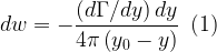
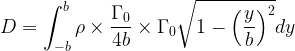
In Prandtl’s classical lifting line theory, a finite wing is replaced by a single spanwise lifting line along which the circulation $\displaystyle \Gamma$ (y) varies; coordinate y denotes the spanwise distance from the center of the wing. At some arbitrary distance y₀ along the lifting line, the trailing vortex system that accompanies the lifting line will induce an infinitesimal velocity dw given by

$\displaystyle dw=-\frac{{\left( {{{d\Gamma }}/{{dy}}} \right)dy}}{{4\pi \left( {{{y}_{0}}-y} \right)}}\,\,\,(1)$

The total velocity w induced by the entire trailing vortex sheet is obtained by integrating (1) over the entire wingspan, that is, from –b to b:

$\displaystyle w\left( {{{y}_{0}}} \right)=-\int_{{-b}}^{b}{{\frac{{\left( {{{d\Gamma }}/{{dy}}} \right)dy}}{{4\pi \left( {{{y}_{0}}-y} \right)}}}}\,\,\,(2)$

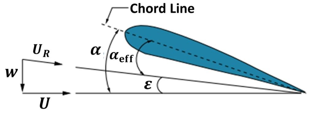
This induced velocity is generally in the downward direction and is termed downwash. Most importantly, downwash has the effect of tilting the resultant wind through an angle $\displaystyle \varepsilon$ such that (Figure 1)

$\displaystyle \varepsilon ={{\tan }^{{-1}}}\left( {\frac{w}{U}} \right)\approx \frac{w}{U}\,\,\,(3)$

where we have used the small-angle approximation because the downwash w is generally much less than the freestream airspeed U. Per equation (3), the downwash reduces the effective incidence so that for the same lift as an equivalent airfoil at incidence $\displaystyle \alpha$ , an incidence of $\displaystyle \alpha$ = $\displaystyle {{\alpha }_{{\text{eff}}}}$ + $\displaystyle \varepsilon$ is required at that section of the airfoil. This modification of angle of attack is a kinematic consequence of downwash, but, as we’ll see in a moment, downwash also has crucial dynamic (i.e., force-related) implications for wing aerodynamics.

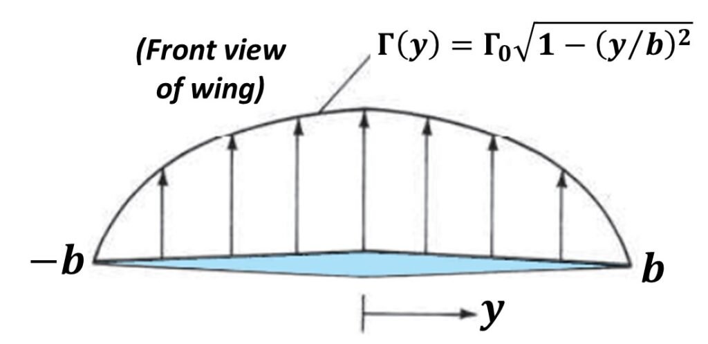
Figure 1. Angles and velocities on an airfoil section. $\displaystyle \alpha$ = Geometric angle of attack; $\displaystyle \varepsilon$ = Induced angle of attack; $\displaystyle {{\alpha }_{{\text{eff}}}}$ = Effective angle of attack. U = Freestream velocity; w = Downwash; U_R = Resultant velocity.

2. Elliptic circulation distribution and downwash

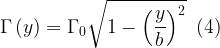
In order to ascertain an induced angle of attack or a lift distribution on a wing, we must know the form of the circulation distribution $\displaystyle \Gamma$ (y). In theoretical terms, the most important such distribution is given by

$\displaystyle \Gamma \left( y \right)={{\Gamma }_{0}}\sqrt{{1-{{{\left( {\frac{y}{b}} \right)}}^{2}}}}\,\,\,(4)$

where $\displaystyle {{\Gamma }_{0}}$ is the circulation at midspan. Since the circulation described by (4) varies elliptically along the span, it is termed an elliptic circulation distribution (Fig. 2).

Figure 2. Elliptically loaded wing.

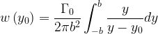
Obtaining the downwash associated with an elliptic distribution is straightforward. The first step is to differentiate (4) with respect to y, giving

$\displaystyle \frac{{d\Gamma }}{{dy}}=-\frac{{{{\Gamma }_{0}}}}{{{{b}^{2}}}}\frac{y}{{\sqrt{{1-{{{{y}^{2}}}}/{{{{b}^{2}}}}\;}}}}$

$\displaystyle \therefore \frac{{d\Gamma }}{{dy}}=-\frac{{{{\Gamma }_{0}}}}{b}\frac{y}{{\sqrt{{{{b}^{2}}-{{y}^{2}}}}}}\,\,\,(5)$

Then, we substitute into (2) and set up the integral

$\displaystyle w\left( {{{y}_{0}}} \right)=\frac{{{{\Gamma }_{0}}}}{{4\pi b}}\int_{{-b}}^{b}{{\frac{y}{{\sqrt{{{{b}^{2}}-{{y}^{2}}}}\left( {y-{{y}_{0}}} \right)}}dy}}\,\,\,(6)$

Adding and subtracting y₀ to the numerator, we can restate (6) as

$\displaystyle w\left( {{{y}_{0}}} \right)=\frac{{{{\Gamma }_{0}}}}{{\pi {{b}^{2}}}}\int_{{-b}}^{b}{{\frac{{\left( {y-{{y}_{0}}} \right)+{{y}_{0}}}}{{\sqrt{{1-{{{{y}^{2}}}}/{{{{b}^{2}}}}\;}}\left( {{{y}_{0}}-y} \right)}}dy}}$

$\displaystyle \therefore w\left( {{{y}_{0}}} \right)=\frac{{{{\Gamma }_{0}}}}{{4\pi b}}\left[ {\int_{{-b}}^{b}{{\frac{{dy}}{{\sqrt{{{{b}^{2}}-{{y}^{2}}}}}}}}+{{y}_{0}}\int_{{-b}}^{b}{{\frac{{dy}}{{\left( {\sqrt{{{{b}^{2}}-{{y}^{2}}}}} \right)\left( {y-{{y}_{0}}} \right)}}}}} \right]\,\,\,(7)$

The first integral in brackets is a standard result that equals $\displaystyle \pi$ , while the second may be replaced with some symbol K, so that

$\displaystyle w\left( {{{y}_{0}}} \right)=\frac{{{{\Gamma }_{0}}}}{{4\pi b}}\left[ {\pi +{{y}_{0}}K} \right]\,\,\,(8)$

Now, as this is a symmetric flight case, the vorticity shed is the same from each side of the wing; therefore, the downwash induced at some spanwise coordinate y₀ in one half of the wing must be the same as that in coordinate –y₀ in the opposite half of the wing. In mathematical terms,

$\displaystyle w\left( {{{y}_{0}}} \right)=w\left( {-{{y}_{0}}} \right)$

$\displaystyle \therefore \frac{{{{\Gamma }_{0}}}}{{4\pi b}}\left[ {\pi +{{y}_{0}}K} \right]=\frac{{{{\Gamma }_{0}}}}{{4\pi b}}\left[ {\pi -{{y}_{0}}K} \right]\,\,\,(9)$

The only way to satisfy this equality is to have K = 0, so that

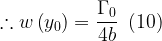
$\displaystyle w\left( {{{y}_{0}}} \right)=\frac{{{{\Gamma }_{0}}}}{{4\pi b}}\times \left( {\pi +0} \right)$

$\displaystyle \therefore w\left( {{{y}_{0}}} \right)=\frac{{{{\Gamma }_{0}}}}{{4b}}\,\,\,(10)$

This important result implies that the downwash on an elliptically loaded wing is constant along the wing span.

3. Lift and drag in an elliptic circulation distribution

According to the Kutta-Joukowski theorem, the contribution to lift L’ at a local airfoil section located at y₀ is given by

$\displaystyle {L}'={{\rho }_{\infty }}{{U}_{\infty }}\Gamma \left( {{{y}_{0}}} \right)\,\,\,(11)$

where $\displaystyle {{\rho }_{\infty }}$ is the freestream air density and $\displaystyle {{U}_{\infty }}$ is the freestream velocity. Replacing $\displaystyle \Gamma$ (y₀) with (4) indicates that the lift distribution of an elliptically loaded wing is also elliptic in nature:

$\displaystyle {L}'={{\rho }_{\infty }}{{U}_{\infty }}{{\Gamma }_{0}}\sqrt{{1-{{{\left( {\frac{y}{b}} \right)}}^{2}}}}\,\,\,(12)$

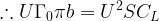
To find the total lift afforded by the circulation distribution, we integrate (12) along the wingspan:

$\displaystyle L=\int_{{-b}}^{b}{{\rho U\Gamma \left( y \right)dy}}$

$\displaystyle \therefore L=\int_{{-b}}^{b}{{\rho U{{\Gamma }_{0}}\sqrt{{1-{{{\left( {\frac{y}{b}} \right)}}^{2}}}}dy}}$

$\displaystyle \therefore L=\rho U{{\Gamma }_{0}}\times \frac{{b\pi }}{2}$

$\displaystyle \therefore L=\rho U{{\Gamma }_{0}}\pi \frac{b}{2}\,\,\,(13)$

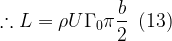
Equation (13) gives the total lift as a function of midspan circulation and wingspan. However, we know that the lift is also given by the classic relationship

$\displaystyle L=\frac{1}{2}\rho {{U}^{2}}S{{C}_{L}}\,\,\,(14)$

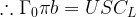
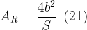
where S = (span $\displaystyle \times$ chord) is the projected area of the wing in the direction normal to the velocity U. Combining (13) and (14) and solving for $\displaystyle {{\Gamma }_{0}}$ , we get

$\displaystyle \rho U{{\Gamma }_{0}}\pi \frac{b}{2}=\frac{1}{2}\rho {{U}^{2}}S{{C}_{L}}$

$\displaystyle \therefore U{{\Gamma }_{0}}\pi b={{U}^{2}}S{{C}_{L}}$

$\displaystyle \therefore {{\Gamma }_{0}}\pi b=US{{C}_{L}}$

$\displaystyle \therefore {{\Gamma }_{0}}=\frac{{{{C}_{L}}US}}{{\pi b}}\,\,\,(15)$

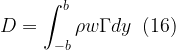
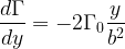
Now, the induced drag caused by the downwash is given by

$\displaystyle D=\int_{{-b}}^{b}{{\rho w\Gamma dy}}\,\,\,(16)$

so that, replacing w with (10) and $\displaystyle \Gamma$ with (4), we write

$\displaystyle D=\int_{{-b}}^{b}{{\rho \times \frac{{{{\Gamma }_{0}}}}{{4b}}\times {{\Gamma }_{0}}\sqrt{{1-{{{\left( {\frac{y}{b}} \right)}}^{2}}}}dy}}$

$\displaystyle \therefore D=\frac{{\rho \Gamma _{0}^{2}}}{{4b}}\int_{{-b}}^{b}{{\sqrt{{1-{{{\left( {\frac{y}{b}} \right)}}^{2}}}}dy}}$

$\displaystyle \therefore D=\frac{{\rho \Gamma _{0}^{2}}}{{4b}}\times \frac{{b\pi }}{2}=\frac{\pi }{8}\rho \Gamma _{0}^{2}\,\,\,(17)$

However, we can replace midspan circulation $\displaystyle {{\Gamma }_{0}}$ with equation (15), giving

$\displaystyle {{D}_{i}}={{\left( {\frac{{{{C}_{L}}US}}{{\pi b}}} \right)}^{2}}\frac{\pi }{8}\rho \,\,\,(18)$

But drag can also be expressed as

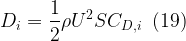
$\displaystyle {{D}_{i}}=\frac{1}{2}\rho {{U}^{2}}S{{C}_{{D,i}}}\,\,\,(19)$

where C_D,I is the induced drag coefficient. Equating (17) to (19) and manipulating, we find that

$\displaystyle {{C}_{{D,i}}}=\frac{{C_{L}^{2}}}{{\pi {{A}_{R}}}}\,\,\,(20)$

where A_R is the aspect ratio of the wing, namely

$\displaystyle {{A}_{R}}=\frac{{4{{b}^{2}}}}{S}\,\,\,(21)$

As can be seen from (20), the variation of C_L with C_D,I for an elliptically loaded airfoil is a parabola, provided the only source of drag is the induced velocity – that is, the downwash. The plot of C_L versus C_D,I is called the polar curve of the airfoil (Fig. 3).

Thus, the induced drag coefficient is directly proportional to the square of the lift coefficient. The dependence of induced drag on lift is not surprising. In phenomenological terms, induced drag is a consequence of the pressure of the wing-tip vortices, which in turn are produced by the difference in pressure between the lower and upper wing surfaces. But the lift is produced by this same pressure difference, hence induced drag is closely related to the production of lift on a finite wing – so much so, in fact, that induced drag is also known as drag due to lift. As Anderson (1984) puts it, an airplane cannot generate lift for free; the induced drag is the price for generation of lift.

In practice, in addition to induced drag there is also profile drag due to skin friction and wake. These phenomena are accounted for by adding a constant C_D,0 to the right-hand side of the drag polar, giving

$\displaystyle {{C}_{D}}={{C}_{{D,0}}}+{{C}_{{D,i}}}$

$\displaystyle \therefore {{C}_{D}}={{C}_{{D,0}}}+\frac{{C_{L}^{2}}}{{\pi {{A}_{R}}}}\,\,\,(22)$

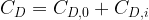
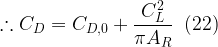
Since profile drag coefficient C_D,0 is independent of C_L, it is also known as the zero-lift drag coefficient. A more rigorous derivation, which is beyond the scope of this post, leads to the modified drag polar

$\displaystyle {{C}_{D}}={{C}_{{D,0}}}+\frac{{C_{L}^{2}}}{{\pi e{{A}_{R}}}}\left( {1+\delta } \right)\,\,\,(23)$

where e is a parameter known as Oswald’s wing efficiency and $\displaystyle \delta$ is a nonnegative parameter that equals zero only in the case of elliptic loading.

Figure 3. Drag polar.

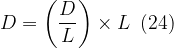
For a wing under elliptic circulation distribution, in straight level flight, what is the condition to minimize drag? We can answer this question using the drag polar (22). Note first that the drag D can be recast as

$\displaystyle D=\left( {\frac{D}{L}} \right)\times L\,\,\,(24)$

But at level flight, lift L equals the weight W, so that

$\displaystyle D=\left( {\frac{D}{L}} \right)\times W\,\,\,(25)$

Thus, for a wing of given weight W, the minimum drag occurs when the drag-to-lift ratio is a minimum (or, equivalently, the lift-to-drag ratio is a maximum). We proceed to restate D/L as

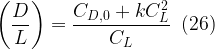
$\displaystyle \left( {\frac{D}{L}} \right)=\frac{{{{C}_{{D,0}}}+kC_{L}^{2}}}{{{{C}_{L}}}}\,\,\,(26)$

where k is a coefficient that condenses all factors that multiply C_L in the drag polar (22). For minimum drag, we differentiate (26) with respect to C_L and set the ensuing expression to zero:

$\displaystyle \frac{{d\left( {{D}/{L}\;} \right)}}{{d{{C}_{L}}}}=0$

$\displaystyle \therefore \frac{d}{{d{{C}_{L}}}}\left[ {\frac{{{{C}_{{D,0}}}+kC_{L}^{2}}}{{{{C}_{L}}}}} \right]=0\,\,\,(27)$

This derivative is straightforward to obtain. We can speed things up using Mathematica:

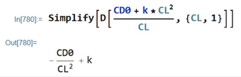
Clearly,

$\displaystyle \frac{d}{{d{{C}_{L}}}}\left[ {\frac{{{{C}_{{D,0}}}+kC_{L}^{2}}}{{{{C}_{L}}}}} \right]=-\frac{{{{C}_{{D,0}}}}}{{C_{L}^{2}}}+k\,\,\,(28)$

Setting this to zero yields

$\displaystyle {{C}_{{D,0}}}=kC_{L}^{2}\,\,\,(29)$

which means that, for minimum drag in an elliptical load distribution, the zero-lift drag coefficient must be equal to the lift-dependent contribution to drag. (The reader is invited to differentiate (28) a second time, substitute from (29), and check that the second derivative at the point in question is positive, which indicates that the point we’ve discussed is indeed a local minimum, not a local maximum.)

Solved example 1

A wing with elliptic loading has span equal to 18 m, planform area 56 m², and moves in level flight at 792 km/h at an altitude where air density equals 0.76 kg/m³. Assuming the induced drag on the wing equals 3400 N, determine:

(a) The lift coefficient.

(b) The downwash velocity.

(c) The wing loading.

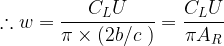
Part a. Before anything else, we compute the aspect ratio A_R:

$\displaystyle {{A}_{R}}=\frac{{4{{b}^{2}}}}{S}=\frac{{4\times {{9}^{2}}}}{{56}}=5.79$

With a flight velocity V = 792 km/h = 220 m/s, we proceed to calculate the induced drag coefficient:

$\displaystyle {{C}_{{D,i}}}=\frac{{{{D}_{i}}}}{{\frac{1}{2}\rho {{U}^{2}}S}}=\frac{{3400}}{{0.5\times 0.76\times {{{220}}^{2}}\times 56}}=0.0033$

Then, the corresponding lift coefficient is determined as

$\displaystyle {{C}_{{D,i}}}=\frac{{C_{L}^{2}}}{{\pi {{A}_{R}}}}\to {{C}_{L}}=\sqrt{{\pi {{A}_{R}}{{C}_{{D,i}}}}}$

$\displaystyle \therefore {{C}_{L}}=\sqrt{{\pi \times 5.79\times 0.0033}}=0.245\leftarrow$

Part b. The downwash for an elliptically loaded wing is constant and given by (10):

$\displaystyle w=\frac{{{{\Gamma }_{0}}}}{{4b}}$

where

$\displaystyle {{\Gamma }_{0}}=\frac{{{{C}_{L}}US}}{{\pi b}}$

so that

$\displaystyle w=\frac{{{{\Gamma }_{0}}}}{{4b}}=\frac{1}{{4b}}\times \frac{{{{C}_{L}}US}}{{\pi b}}=\frac{{{{C}_{L}}V\left( {2b\times c} \right)}}{{\pi b\times 4b}}$

$\displaystyle \therefore w=\frac{{{{C}_{L}}U}}{{\pi \times \left( {{{2b}}/{c}\;} \right)}}=\frac{{{{C}_{L}}U}}{{\pi {{A}_{R}}}}$

$\displaystyle \therefore w=\frac{{0.245\times 220}}{{\pi \times 5.79}}=2.96\,\ \text{m/s}\leftarrow$

Part c. In level flight, lift equals weight, or

$\displaystyle W=L=\frac{1}{2}\rho {{U}^{2}}S{{C}_{L}}$

$\displaystyle \therefore W=\frac{1}{2}\times 0.76\times {{220}^{2}}\times 56\times 0.245=252,000\,\ \text{N}$

Lastly, the wing loading is

$\displaystyle \frac{W}{S}=\frac{{252,000}}{{56}}=4500\,\,\text{N/}{{\text{m}}^{2}}\leftarrow$

Solved example 2

Obtain an expression for the downward induced velocity behind a wing of span 2b at a point y from the center of the span, the circulation around the wing at any point y being $\displaystyle \Gamma$ . If the circulation is parabolic, that is,

$\displaystyle \Gamma ={{\Gamma }_{0}}\left( {1-\frac{{{{y}^{2}}}}{{{{b}^{2}}}}} \right)$

calculate the value of the induced velocity w at midspan, and compare this value with that obtained when the same lift is distributed elliptically.

Solution. The derivative of the given span circulation we were given is

$\displaystyle \frac{{d\Gamma }}{{dy}}=-2{{\Gamma }_{0}}\frac{y}{{{{b}^{2}}}}$

so that, substituting in (2),

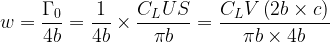
$\displaystyle w\left( {{{y}_{0}}} \right)=\frac{{{{\Gamma }_{0}}}}{{2\pi {{b}^{2}}}}\int_{{-b}}^{b}{{\frac{y}{{y-{{y}_{0}}}}dy}}$

At midspan this reduces to

$\displaystyle w\left( 0 \right)=\frac{{{{\Gamma }_{0}}}}{{2\pi {{b}^{2}}}}\int_{{-b}}^{b}{{\frac{y}{{y-0}}dy}}$

$\displaystyle \therefore w\left( 0 \right)=\frac{{{{\Gamma }_{0}}}}{{2\pi {{b}^{2}}}}\int_{{-b}}^{b}{{dy}}$

$\displaystyle \therefore {{w}_{{\text{par}}}}\left( 0 \right)=\frac{{{{\Gamma }_{0}}}}{{\pi b}}\,\,\,(30)$

It is pertinent to ask how this compares with an elliptically loaded wing with the same lift. Note first that the lift for the parabolic circulation distribution is such that

$\displaystyle L=\rho U{{\Gamma }_{0}}\int_{{-b}}^{b}{{\left( {1-\frac{{{{y}^{2}}}}{{{{b}^{2}}}}} \right)dy}}=\rho U{{\Gamma }_{0}}\times \frac{{4b}}{3}$

$\displaystyle \therefore L=\frac{{4\rho U{{\Gamma }_{0}}b}}{3}$

In contrast, the lift for an elliptically loaded wing is given by eq. (13), namely

$\displaystyle {{L}_{e}}=\rho U{{\Gamma }_{{0,e}}}\pi \frac{b}{2}$

For the same lift in both cases, we must have

$\displaystyle \frac{{4\rho U{{\Gamma }_{0}}b}}{3}=\rho U{{\Gamma }_{{0,e}}}\pi \frac{b}{2}$

$\displaystyle \therefore {{\Gamma }_{{0,e}}}=\frac{{8{{\Gamma }_{0}}}}{{3\pi }}\,\,(31)$

Further, noting that

$\displaystyle {{w}_{e}}=\frac{{{{\Gamma }_{{0,e}}}}}{{4b}}$

and substituting from (30) and (31), we get

$\displaystyle {{w}_{e}}=\frac{{{{\Gamma }_{{0,e}}}}}{{4b}}=\frac{1}{{4b}}\times \frac{{8{{\Gamma }_{0}}}}{{3\pi }}=\frac{2}{3}\times \frac{{{{\Gamma }_{0}}}}{{\pi b}}$

$\displaystyle \therefore {{w}_{e}}=\frac{2}{3}{{w}_{{\text{par}}}}$

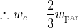
which implies that the downwash associated with an elliptically loaded wing is 2/3 of the downwash of a parabolically loaded wing.

References

ANDERSON, J.D. Jr. (1984). Fundamentals of Aerodynamics. New York: McGraw-Hill.
HOUGHTON, E.L., CARPENTER, P.W., COLLICOTT, S.H. and VALENTINE, D.T. (2017). Aerodynamics for Engineering Students. 7th edition. Oxford: Butterworth-Heinemann.
RATHAKRISHNAN, E. (2013). Theoretical Aerodynamics. Hoboken: John Wiley and Sons.

Elliptic Circulation Distribution and Downwash

Subscribe to our Mailing List!

Featured Posts

A Primer on NAND Flash Memories

Solidification Time and Chvorinov’s Rule

Step-Growth Polymerization, the Carothers Equation, and the Flory-Schulz Distribution

More Articles

Flow in Noncircular Ducts

Solidification Time and Chvorinov’s Rule

Fields of Study

More

© 2024 Montogue Quiz

Subscribe to
our Mailing List!

Subscribe to our Mailing List!

Subscribe to receive our latest materials in your inbox.

Homework Help

© 2024 Montogue Quiz

Subscribe to our Mailing List!