Fatigue Life and the Palmgren-Miner Rule

1. The Palmgren-Miner rule

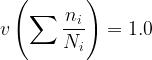
Any discussion on fatigue theory would be incomplete without considering variable-amplitude loading. Many structures are subjected to a range of load fluctuations, mean levels, and frequencies. The task then is to predict, based on constant-amplitude test data, the life of a component subjected to a variable load history. A number of cumulative damage theories, proposed during the past few decades, describe the relative importance of stress interactions and the amount of damage – plastic deformation, crack initiation, and propagation – introduced to a component. The simplest mathematical formulation of cumulative damage fatigue is the relation

$\displaystyle \sum\limits_{{i=1}}^{k}{{\frac{{{{n}_{i}}}}{{{{N}_{i}}}}}}=1$

Here, $\displaystyle {{n}_{i}}$ is the number of cycles applied at the i-th stress level $\displaystyle {{\sigma }_{i}}$ , $\displaystyle {{N}_{i}}$ is the fatigue life at $\displaystyle {{\sigma }_{i}}$ , and k is the number of stress levels in the block loading spectrum. The ratio of the number of cycles at a given stress level to the fatigue life is sometimes called the cycle ratio. In practical terms, the equation above states that fatigue failure occurs when the sum of the cycle ratios amounts to one.

This relationship was proposed by A. Palmgren in Sweden in the 1920s for predicting the life of ball bearings, and then it was applied in a more general context by B. F. Langer in 1937. However, the rule was not widely known or used until its appearance in a paper by M. A. Miner. published in 1945.

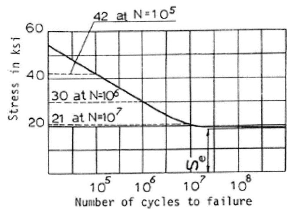
In a typical application of the Miner rule, the values of n are usually given, and N can be estimated from a stress-life curve – or S–N curve, as it is more commonly known – a graph that provides the number of cycles of failure associated with each stress level. One such curve is shown below. This technique is illustrated in the following example.

Example 1

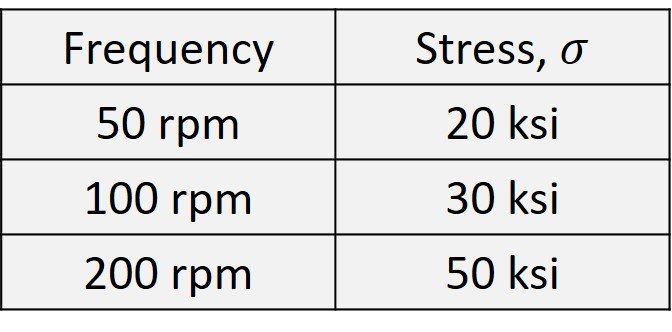
A short-life bearing component in a rotating machinery undergoes cyclic dynamic loads due to synchronous rotor vibration. The rotor was operated at 50 rpm for 13 hrs and 20 min, then the speed was increased to 100 rpm and the rotor was run for an additional 8 hrs 20 min. Assuming the graph and numerical data of the following figure, estimate the number of operational fatigue cycles and maximum run time at 200 rpm so that a cumulative damage factor of 0.75 is not exceeded.

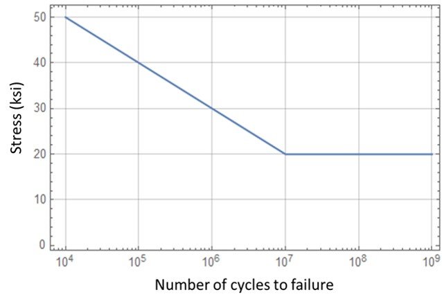
Referring to the S-N curve, we see that the number of cycles to failure at the abovementioned maximum stresses are $\displaystyle N$ = $\displaystyle {{10}^{7}}$ for $\displaystyle {{\sigma }_{{\max }}}$ = 20 ksi and $\displaystyle N$ = $\displaystyle {{10}^{6}}$ for $\displaystyle {{\sigma }_{{\max }}}$ = 30 ksi. The number of cycles the component was subjected to is 800 $\displaystyle \times$ 50 = 40,000 cycles at 20 ksi and 500 $\displaystyle \times$ 100 = 50,000 cycles at 30 ksi. In view of the Palmgren-Miner rule, we may write

$\displaystyle \frac{n}{N}+\frac{{40,000}}{{10,000,000}}+\frac{{50,000}}{{1,000,000}}=0.75$

$\displaystyle \frac{n}{N}=0.686$

Operation at 200 rpm implies a stress of $\displaystyle {{\sigma }_{{\max }}}$ = 50 ksi, which in turn corresponds to a number of cycles to failure of $\displaystyle N$ = $\displaystyle {{10}^{4}}$ . Accordingly, the corresponding number of operational cycles is

$\displaystyle n={{10}^{4}}\times 0.686=6860\,\,\text{cycles}$

The maximum allowable service life at 200 rpm follows as

$\displaystyle t=\frac{{6860\,\,\text{cycles}}}{{200\,\,\text{cycles/min}}}=34.3\,\,\text{min}\leftarrow$

That is, the component can operate at 200 rpm for about 34 minutes without exceeding the cumulative damage factor limit of 0.75.

2. More on fatigue life analysis

Dowling (2013) presents a slightly more elaborated analysis of fatigue life with the Miner rule. In his approach, the amplitude of stress is stated as a function of the number of cycles to failure, $\displaystyle {{N}_{f}}$ , in an equation of the form

$\displaystyle {{\sigma }_{a}}={{{\sigma }'}_{f}}{{\left( {2{{N}_{f}}} \right)}^{b}}$

where $\displaystyle {{{\sigma }'}_{f}}$ and $\displaystyle b$ are parameters that depend on the material. The life of a specimen is evaluated on the basis of the completely reversed stress, $\displaystyle {{\sigma }_{{ar}}}$ , which can be estimated with the Smith, Watson and Topper (SWT) equation

$\displaystyle {{\sigma }_{{ar}}}=\sqrt{{{{\sigma }_{{\max }}}{{\sigma }_{a}}}}$

where $\displaystyle {{\sigma }_{{\max }}}$ is the maximum stress amplitude.

A particular sequence of loading may be repeatedly applied to an engineering component, or, for a continually varying load history, a typical sample may be available. Under these circumstances, it is convenient to sum cycle ratios over one repetition of a given load sequence and then multiply the result by the number of repetitions required for the summation to reach unity:

$\displaystyle v\left( {\sum\limits_{\,}^{\,}{{\frac{{{{n}_{i}}}}{{{{N}_{i}}}}}}} \right)=1.0$

where $\displaystyle v$ is the number of repetitions to failure. Another example follows.

Example 2

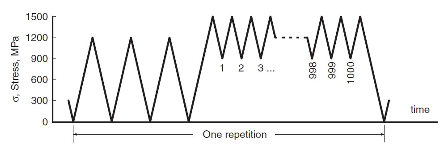
In a location of interest in an engineering component, the material is repeatedly subjected to the uniaxial stress history shown in the following figure. The component is made of SAE 4142 steel. Estimate the number of repetitions necessary to cause fatigue failure. For this steel, $\displaystyle {{{\sigma }'}_{f}}$ = 1940 MPa and b = –0.0762.

To begin, we invoke the SWT equation,

$\displaystyle {{\sigma }_{{ar}}}=\sqrt{{{{\sigma }_{{\max }}}{{\sigma }_{a}}}}$

However, the completely reversed stress is also expressed as

$\displaystyle {{\sigma }_{{ar}}}={{{\sigma }'}_{f}}{{\left( {2{{N}_{f}}} \right)}^{b}}$

Equating the two previous relations, we have

$\displaystyle \sqrt{{{{\sigma }_{{\max }}}{{\sigma }_{a}}}}={{{\sigma }'}_{f}}{{\left( {2{{N}_{f}}} \right)}^{b}}$

$\displaystyle \therefore {{N}_{f}}=\frac{1}{2}{{\left( {\frac{{\sqrt{{{{\sigma }_{{\max }}}{{\sigma }_{a}}}}}}{{{{{{\sigma }'}}_{f}}}}} \right)}^{{{1}/{b}\;}}}\,\,\,(1)$

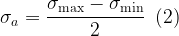
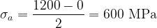
The mean nominal stress range is expressed as

$\displaystyle {{\sigma }_{a}}=\frac{{{{\sigma }_{{\max }}}-{{\sigma }_{{\min }}}}}{2}\,\,\,(2)$

Consider, for example, the segment of the uniaxial stress history highlighted below.

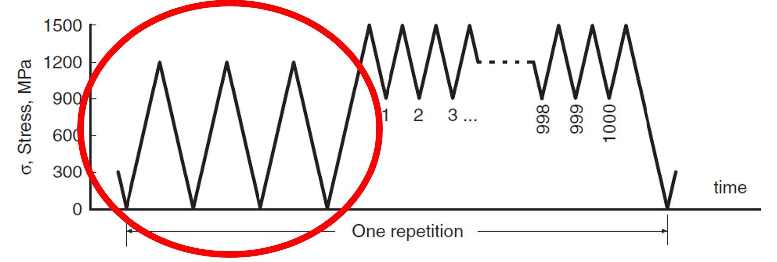
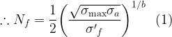
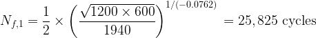
By inspection, it is easy to see that $\displaystyle {{\sigma }_{{\max }}}$ = 1200 MPa and $\displaystyle {{\sigma }_{{\min }}}$ = 0. Substituting in equation (2) brings to

$\displaystyle {{\sigma }_{a}}=\frac{{1200-0}}{2}=600\,\,\text{MPa}$

Then, plugging this result into equation (1), the number of cycles to failure is found as

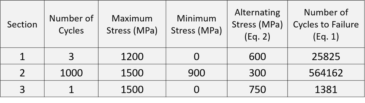
$\displaystyle {{N}_{{f,1}}}=\frac{1}{2}\times {{\left( {\frac{{\sqrt{{1200\times 600}}}}{{1940}}} \right)}^{{{1}/{{\left( {-0.0762} \right)}}\;}}}=25,825\,\,\text{cycles}$

Proceeding similarly with the other segments of the loading history, the following table is prepared.

Let $\displaystyle \nu$ be the number of cycles to failure. Appealing to the Miner rule, we write

$\displaystyle v\left( {\frac{{{{n}_{1}}}}{{{{N}_{{f,1}}}}}+\frac{{{{n}_{2}}}}{{{{N}_{{f,2}}}}}+\frac{{{{n}_{3}}}}{{{{N}_{{f,3}}}}}} \right)=1$

Substituting the numerical data and solving for $\displaystyle \nu$ ,

$\displaystyle \nu \left( {\frac{3}{{25,825}}+\frac{{1000}}{{564,162}}+\frac{1}{{1381}}} \right)=1.0$

$\displaystyle \therefore v=383\,\,\text{repetitions}\leftarrow$

That is, the number of repetitions necessary to cause fatigue failure is 383.

Go further

The problems discussed in this post are adapted from our free quiz on fatigure of materials theory, which you can find here. Students may also be interested in our free quiz on elementary fracture mechanics.

References

• DOWLING, N. (2013). Mechanical Behavior of Materials – International Edition. 4th edition. Upper Saddle River: Pearson.

• HERTZBERG, J., VINCI, R. and HERTZBERG, J. (2013). Deformation and Fracture Mechanics of Engineering Materials. 5th edition. Hoboken: John Wiley and Sons.

• SHUKLA, A. (2005). Practical Fracture Mechanics in Design. 2nd edition. New York: Marcel Dekker.

Fatigue Life and the Palmgren-Miner Rule

Subscribe to our Mailing List!

Featured Posts

A Primer on NAND Flash Memories

Solidification Time and Chvorinov’s Rule

Step-Growth Polymerization, the Carothers Equation, and the Flory-Schulz Distribution

More Articles

Size Reduction, the Three Laws of Comminution, and the Bond Equation

Murray’s Law and the Analysis of Arterial Bifurcations

Fields of Study

More

© 2024 Montogue Quiz

Subscribe to
our Mailing List!

Subscribe to our Mailing List!

Subscribe to receive our latest materials in your inbox.

Homework Help

© 2024 Montogue Quiz

Subscribe to our Mailing List!