

1. Introduction
The preservation of food by refrigeration is based on a very general principle of physical chemistry: molecular mobility is reduced and, consequently, chemical reactions and biological processes are slowed down at low temperature (Berk, 2009). Simply put, foods are frozen to depress microbial and enzymatic activity so that quality is not compromised during storage.
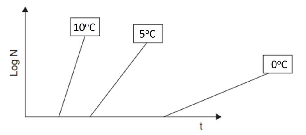
Figure 1 is a schematic representation of the relationship between storage temperature and the microbial load of a certain food. Kinetically, a lower temperature is associated with a longer induction period (lag phase) and a slower growth rate in the logarithmic phase. Due to these two factors, the microbial count after a given frozen storage time is substantially lower than observed for the same food in unrefrigerated conditions. As a result, there is great practical value in understanding the thermophysical mechanics of freezing processes and their associated metrics, most notably the freezing time required to attain a certain temperature, usually several degrees below zero. A sound understanding of freezing time enables stakeholders to improve food safety, minimize power consumption, and so forth.
Figure 1. Variation of logarithm of microbial population as a function of time for three hypothetical temperatures.
However, foods undergoing freezing release latent heat over a range of temperatures, as freezing does not occur at a unique temperature. What’s more, the thermal properties of foods, including specific heat and thermal conductivity, are not constant with temperature. In view of these and other traits of refrigeration processes, the development of realistic models for freezing time of foods is made difficult, and engineers must instead rely on simplified analytical or computationally intensive numerical methods. In this post, we briefly visit two food freezing time models: The first, Plank’s equation, is mainly of historical value but nonetheless constitutes an interesting preamble to more complicated models; the second, the simplified Pham model, was introduced in the 1980s and offers a combination of reasonable accuracy and quick calculation that few other models in the literature can rival.
2. Plank’s equation
Let us consider a slab-shaped foodstuff of constant thickness z being exposed to a cold medium at temperature T∞, which is below the freezing point Tf of the food. The following assumptions are made:
- The sides of the slab are perfectly insulated, or the slab has infinite area, so that the heat flux is normal to its faces.
- The phase change takes place at a single sharp temperature Tf, at which latent heat
(J/kg) is released.
- The sensible specific heat of the material is zero both above and below the freezing point.
- A third-kind or convective boundary condition applies at the surface.
Figure 2. Infinite slab-shaped foodstuff being frozen.
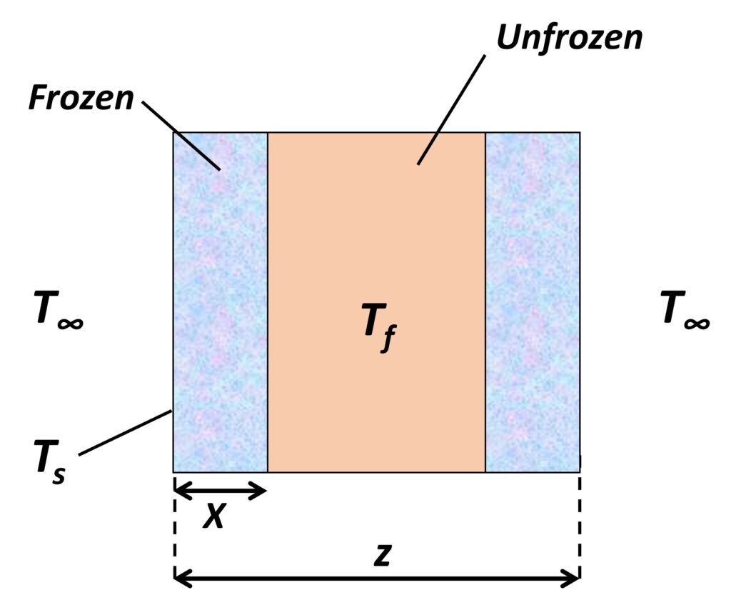
As the material has no sensible specific heat, it will immediately fall to the freezing point throughout. A freezing front will form at the surface at time t = 0, then advance towards the center (Figure 2). Per Fourier’s law, heat conduction through the frozen region is given by

where kf is the thermal conductivity of the frozen food, A is the area of the surface exposed to the cooling medium (usually air), Ts is the temperature of the surface, Tf is the freezing temperature of the food material, and X is the thickness of the freezing front. In turn, convective heat transfer at the surface is governed by Newton’s law of cooling:

where h is the convective heat transfer coefficient and T∞ is the temperature of the cooling medium. With reference to the two previous equations, the thermal resistance encountered by the food is

The overall heat conduction rate is

This rate of heat transfer should be equal to the rate of release of latent heat of freezing, namely
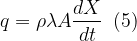
where 

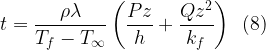
so that, separating variables and integrating,


This relationship is known as Plank’s equation; it was originally proposed by R.Z. Plank in 1913 and later updated in a 1941 paper. In a more general form, the equation can be restated as
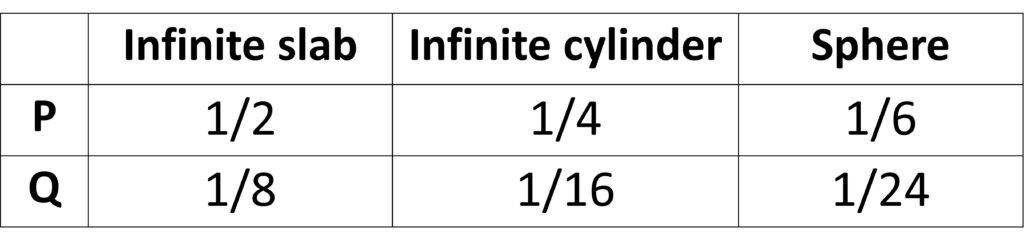
where P and Q are constants that depend on the geometry of the food, as summarized in Table 1.
Table 1. Parameters P and Q for use with Plank’s equation.
When the shape of the food is not simple, the easiest approach is to calculate the freezing time tslab for an infinite slab with the same thickness as the smallest dimension of the food, then apply a shape factor E:

Shape factors have been found for many regular shapes, including rectangular rods, finite cylinders, and ellipsoids; see Pham (2008) for details.
Pham (1986, 2014) showed that Plank’s solutions can be written in the following general form for the three basic shapes:
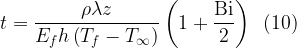
where the shape factor Ef is 1 for slabs, 2 for infinite cylinders, and 3 for spheres. In turn, Bi is the Biot number based on frozen food thermal conductivity; mathematically,
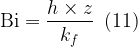
We observe that for the three basic shapes, Ef is equal to the ratio Az/V, where A is the surface area of the food and V is the volume. Accordingly, (10) can be restated as
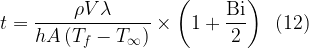
The first term on the right-hand side of (12) is the freezing time for an object with zero internal resistance to heat transfer, while the second term, (1 + Bi/2), is a correction factor for finite conductivity, or thermal resistance. During freezing, the latent heat flux has to traverse a distance z/2 as it reaches the center of the slab, so the average internal resistance to heat transfer is z/2kf. It follows that Bi/2 = hz/2kf is an estimate of the ratio of internal to external (surface) resistances to heat transfer during the freezing process.
Pham (2014) notes that the freezing time achieves two limiting values as the Biot number becomes very high or very low. If Bi 


so the freezing time becomes proportional to the square of size. If, on the other hand, Bi

so the freezing time becomes linearly proportional to size.
Pham (2014) advises that refrigeration engineers should be aware of the Biot number of their processes. If Bi is substantially greater than unity – that is, if internal resistance controls heat transfer – there is little use in modifying the heat transfer coefficient via, say, increasing air velocity, and the engineer should instead try to reduce the thickness of the food (if possible). If, on the other hand, Bi is much lower than unity, surface resistance controls and effort should be made to increase the convective heat transfer coefficient. Pham (2014) closes by noting that comminution of the food into smaller units may increase the surface area to volume ratio A/R and reduce freezing time irrespective of the Biot number employed.
Solved example 1
Meat balls of diameter equal to 5 cm are to be frozen in a cold-air environment at ‒35oC. The meat balls have density of 1150 kg/m3, water content equal to 76%, and begin to freeze at a temperature of approximately ‒2oC. The thermal conductivity of frozen meat is 1.2 W/m-K and the convective heat transfer coefficient for the air-meat ball interface is 20 W/m2-K. Taking
Answer. This is a straightforward application of Plank’s equation; substituting the pertaining data and noting that, for a sphere, P = 1/6 and Q = 1/24, we have


The meat ball will be frozen within less than one hour and 15 minutes.
3. Pham’s simplified method
In practice, the Plank equation is not accurate because it neglects several relevant phenomena, such as:
- The food may not be at the freezing point initially.
- Its shape may not be one of the three simple shapes and may be more complicated or asymmetrical.
- Real foods freeze gradually over a range of several degrees.
In the 1980s, Q.T. Pham, arguably the world’s most prominent expert on food freezing, published a simple formula that yields better predictions of freezing time than the Plank equation. Pham’s (1986) formula is

where 

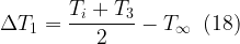
where cpu is the specific heat of the unfrozen food, Ti is the initial temperature and T3 is the mean freezing temperature, which can be estimated as

in which T is the final freezing temperature and T∞ is the temperature of the cooling medium, both in oC. Next, temperature change
Next, heat term

where
The Biot number in Pham’s equation is Bi = hz/kf, where z is a length scale equal to the thickness of an infinite slab, the diameter of an infinite cylinder, or a sphere’s diameter. For brick-shaped foods, Pham recommends the equation

where W1 and W2 are the shortest and second-shortest dimensions of the brick, respectively.
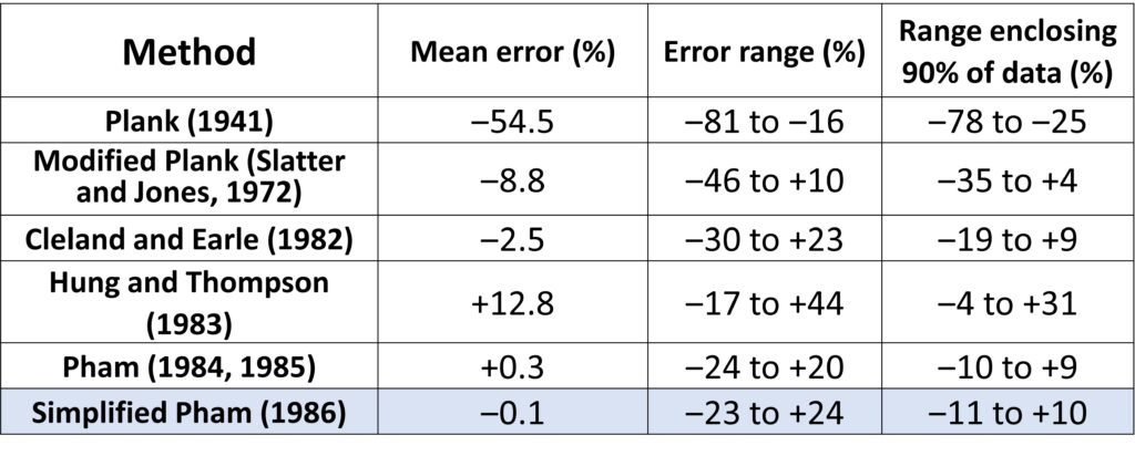
In spite of its simplicity, Pham’s method is satisfactorily accurate. Table 2 summarizes the errors verified when this approach was used to compute freezing times for four published sets of freezing data encompassing 283 data points. The data cover a wide range of test materials (including lean beef, ground beef, potato and carp), Biot numbers (0.045 to 21), and shapes (slabs, cylinders, and spheres). It can be seen that Pham’s method exhibits mean errors lower than most other models available at the time of its publication.
Table 2. Accuracy of several freezing time models reviewed by Pham (1986). See Pham’s paper for the respective references.
Solved example 2
Consider a beef slab of 0.12-m thickness and infinite area. The following data are given:
- Initial food temperature, Ti = 4oC
- Final frozen product temperature, T = ‒20oC
- Ambient temperature, T∞ = ‒33oC
- Surface heat convection coefficient, h = 35 W/m2-K
- Thermal conductivity of frozen beef, kf = 1.75 W/m-K
- Density,
- Moisture content, 78%
- Latent heat of freezing,
- Specific heat of the frozen product, cpf = 2.5 kJ/kg-K
- Specific heat of the unfrozen product, cpu = 3.6 kJ/kg-K
Use the simplified Pham model to calculate the freezing time.
Answer. The reference dimension for the slab is z = 0.12 m, so the Biot number becomes
Next, we compute temperature T3:

and
![\displaystyle \Delta {{H}_{1}}={{c}_{{pu}}}\left( {{{T}_{i}}-{{T}_{3}}} \right)=3600\times \left[ {4-\left( {-6.93} \right)} \right]=39,350\,\,\text{J/kg}](https://s0.wp.com/latex.php?latex=%5Cdisplaystyle+%5CDelta+%7B%7BH%7D_%7B1%7D%7D%3D%7B%7Bc%7D_%7B%7Bpu%7D%7D%7D%5Cleft%28+%7B%7B%7BT%7D_%7Bi%7D%7D-%7B%7BT%7D_%7B3%7D%7D%7D+%5Cright%29%3D3600%5Ctimes+%5Cleft%5B+%7B4-%5Cleft%28+%7B-6.93%7D+%5Cright%29%7D+%5Cright%5D%3D39%2C350%5C%2C%5C%2C%5Ctext%7BJ%2Fkg%7D&bg=ffffff&fg=000&s=1&c=20201002)
Then, noting that 


Next, we calculate


Appealing to the Pham equation, we have

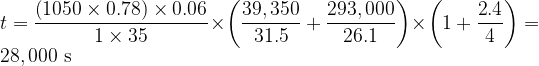

The food should be frozen to the desired temperature within approximately 7 hours and 45 minutes.
References
- BERK, Z. (2009). Food Process Engineering and Technology. London: Academic Press.
- PHAM, Q.T. (1986). Simplified equation for predicting the freezing time of foodstuffs. Int. J. Food Technol., 21(2), 209 – 219. DOI: 10.1111/j.1365-2621.1986.tb00442.x
- PHAM, Q.T. (2008). Modelling of freezing processes. In: EVANS, J.A. (Ed.). Frozen Food Science and Technology. Oxford: Blackwell.
- PHAM, Q.T. (2014). Food Freezing and Thawing Calculations. Berlin/Heidelberg: Springer.
- SUN, D.-W. (Ed.) (2012). Handbook of Frozen Food Processing and Packaging. 2nd edition. Boca Raton: CRC Press.