Plasmas and MHD Shocks

1. Introduction

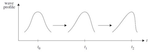
In the jargon of hydrodynamic transport phenomena, a ‘shock’ is a discontinuity separating two different regions in an otherwise continuous medium (Kallenrode, 2004). It is associated with a disturbance moving faster than the rate of signal propagation in the environment, such as an airplane traveling at a speed greater than the speed of sound. Shocks arise by means of a wave steepening mechanism (Figure 1) in which a rapidly speeding agent generates compression waves and eventually outstrips the wave fronts themselves, generating a sudden, non-adiabatic change of state.

Figure 1. Illustration of wave-front steepening in propagation of a compression wave.

In ordinary gas dynamics, the shock is a transition associated with supersonic flow behind the shock and subsonic flow in front of it. Given the upstream state of the flow, a question arises: what are the thermomechanical variables, such as velocity, density, pressure, temperature and entropy, on the downstream, subsonic, side of the shock? In neutral gas dynamics, this question is answered by the Rankine-Hugoniot relations, and the behavior of the transition is straightforwardly characterized the sound speed, c. In MHD shocks, there are three characteristic velocities, as we will find out shortly, which renders the analysis more complex and nuanced than in models of hydrodynamic shocks.

While the study of non-conducting (i.e., unmagnetized and electrically neutral) shocks has occupied researchers since the days of pioneers such as Hugoniot and Prandtl in the late 19^th/early 20^th centuries, research on magnetohydrodynamic shocks is more recent. Experimental work with plasmas began in the late 1920s and accelerated in the early post-war era; starting in the 1950s, research on magnetohydrodynamic shocks blossomed as a byproduct of advanced countries’ growing interest in fusion power and universities’ rapidly expanding space research programs. Two classic papers on MHD shocks are Herlofson (1950) and de Hoffmann and Teller (1950).

2. De Hoffmann-Teller frame

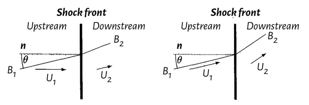
Needless to say, the crucial difference between a MHD shock and an ordinary shock is the magnetic field. When casting the conservation equations for a MHD shock, plasma scientists often make use of the de Hoffmann-Teller frame, Figure 2. In the normal incidence frame, the upstream plasma flow is normal to the shock and oblique to the magnetic field. The downstream flow is oblique to both the magnetic field and shock normal. In the de Hoffmann-Teller frame, the plasma flow is parallel to the magnetic field on both sides of the shock and the U $\displaystyle \times$ B induction field in the shock front vanishes.

Figure 2. Frames of reference for MHD shocks: normal incidence frame (left) and de Hoffmann-Teller frame (right).

3. Jump conditions and shock adiabatic

The conservation laws that relate the thermomechanical variables upstream and downstream of a discontinuity are known as jump conditions. The jump conditions associated with an MHD shock derive (1) from ideal MHD equations for mass, momentum, and energy conservation; and (2) from the requirement, afforded by Maxwell’s equations, that the tangential component of the electric field and the normal component of the magnetic field must be continuous across the discontinuity. We may write down a variation in some thermomechanical variable $\displaystyle \phi$ from upstream of the shock (subscript ‘1’) to downstream of the shock (subscript ‘2’) with the simplified notation

$\displaystyle \left\{ \phi \right\}={{\phi }_{2}}-{{\phi }_{1}}\,\,\,\,\,\mathbf{(1)}$

Accordingly, we have:

Conservation of mass

$\displaystyle \left\{ {{{\rho }_{m}}{{U}_{n}}} \right\}=0\,\,\,\,\,\mathbf{(2)}$

Conservation of momentum flux 1

$\displaystyle \left\{ {{{\rho }_{m}}U_{n}^{2}+P+\frac{{B_{t}^{2}}}{{2{{\mu }_{0}}}}} \right\}=0\,\,\,\,\,\left( \mathbf{3} \right)$

Conservation of momentum flux 2

$\displaystyle \left\{ {{{\rho }_{m}}{{U}_{n}}{{\mathbf{U}}_{t}}-{{B}_{n}}\frac{{{{B}_{t}}}}{{{{\mu }_{0}}}}} \right\}=0\,\,\,\,\,\left( \mathbf{4} \right)$

Conservation of energy

$\displaystyle \left\{ {\left( {\frac{1}{2}{{\rho }_{m}}{{U}^{2}}+h+\frac{{{{B}^{2}}}}{{{{\mu }_{0}}}}} \right){{U}_{n}}-\left( {\mathbf{U}\cdot \mathbf{B}} \right)\frac{{{{B}_{n}}}}{{{{\mu }_{0}}}}} \right\}=0\,\,\,\,\,\mathbf{(5)}$

Continuity of tangential component of electric field (recall that $\displaystyle \mathbf{E}$ = $\displaystyle -\mathbf{U}\times \mathbf{B}$ )

$\displaystyle \left\{ {{{\mathbf{U}}_{n}}\times {{\mathbf{B}}_{t}}+{{\mathbf{U}}_{t}}\times {{\mathbf{B}}_{n}}} \right\}=0\,\,\,\,\,\left( \mathbf{6} \right)$

Continuity of normal component of magnetic field

$\displaystyle \left\{ {{{B}_{n}}} \right\}=0\,\,\,\,\,\left( \mathbf{7} \right)$

In these relations, $\displaystyle {{\rho }_{m}}$ is the mass density of the plasma, $\displaystyle {{U}_{n}}$ is the velocity component normal to the discontinuity surface, $\displaystyle {{U}_{t}}$ is the tangential component of velocity, P is pressure, B_n is the normal component of magnetic field, B_t is the tangential component of magnetic field, h is enthalpy and is the vacuum magnetic permeability. Note that when B = 0 the jump conditions reduce to the Hugoniot-Rankine relations for a neutral hydrodynamic shock.

As the reader will surely have noticed, we had nothing to say about the entropy of this system. For brevity, we simply note that entropy increases across a MHD shock, and that this increase is indicative of irreversible dissipative processes across the shock. Chapter 16 in Somov (2012) covers the entropy issue in much greater detail.

The formulation of the MHD shock problem characterized by equations (2)–(7) has one more variable than equations, hence we must introduce a new parameter to make the system tractable. Following Gurnett and Bhattacharjee (2017), we introduce the shock strength or compression ratio r, which is the ratio of the downstream to the upstream plasma densities,

$\displaystyle r=\frac{{{{\rho }_{{m2}}}}}{{{{\rho }_{{m1}}}}}\,\,\,\,\,\left( \mathbf{8} \right)$

This leads to closure of the problem. We also introduce two more indispensable dimensionless quantities, namely

$\displaystyle {{M}_{A}}=\frac{{{{U}_{n}}}}{{{{V}_{{An}}}}}\,\,\,\,\,\left( \mathbf{9} \right)$

and

$\displaystyle {{M}_{S}}=\frac{{{{U}_{n}}}}{{{{V}_{S}}}}\,\,\,\,\,\mathbf{(10)}$

Parameter M_A is the Alfvén Mach number, defined as the ratio of the normal component of flow velocity to the normal component of the Alfvén velocity. In turn, parameter M_S is the sonic Mach number, defined as the ratio of the normal component of flow velocity to the sound speed. (We won’t use these Mach numbers directly, but they are crucial in other aspects of MHD shock theory and the reader interested in MHD shocks should be aware of their importance in hydromagnetic transport phenomena.) One last parameter essential to our analysis is the angle $\displaystyle \theta$ between the magnetic field and the shock normal, which we’ve already seen in Figure 2,

$\displaystyle \tan \theta =\frac{{{{B}_{t}}}}{{{{B}_{n}}}}\,\,\,\,\,\mathbf{(11)}$

Equipped with these quantities, we may write down the shock adiabatic for a plasma with heat capacity ratio $\displaystyle \gamma$ ,

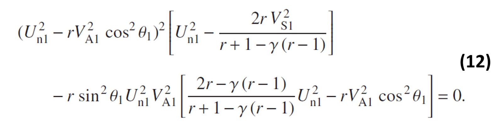
This equation, albeit long, is merely an expression for the propagation speed of the shock as a function of other upstream variables (designated with a subscript ‘1’) and plasma parameters (compression ratio r and heat capacity ratio $\displaystyle \gamma$ ). The shock adiabatic is akin to the so-called dispersion relations found in linear wave and oscillation theory, except the propagation speed now depends on the wave amplitude. Equation (12) is a cubic equation in $\displaystyle U_{{n1}}^{2}$ ; accordingly, three pairs of roots exist, corresponding to three pairs of oppositely propagating shocks. In order of increasing speeds, these shocks are called the slow, intermediate, and fast MHD shocks. Figure 3 depicts the three possibilities of the magnetic field orientation behind a shock moving at an oblique angle to the magnetic field of the plasma ahead.

Figure 3. Changes in magnetic field direction (arrow) from ahead (upstream) to behind (downstream) an MHD shock.

4. Special cases

4.1. Weak shock limit

In the weak shock limit, the density of the plasma upstream and downstream of the shock is equal, so the shock strength is r = 1. In this case, the shock adiabatic takes the form

$\displaystyle \left( {U_{{n1}}^{2}-V_{{A1}}^{2}{{{\cos }}^{2}}{{\theta }_{1}}} \right)\left[ {U_{{n1}}^{4}-U_{{n1}}^{2}\left( {V_{{A1}}^{2}+V_{{S1}}^{2}} \right)+V_{{S1}}^{2}V_{{A1}}^{2}} \right]=0\,\,\,\,\,\mathbf{(13)}$

which is found to be identical to the dispersion relation for small-amplitude waves in an MHD fluid, except that in our results the shock speed U_n1 substitutes the phase speed. MHD shocks usually travel faster than the linear MHD modes. However, as the compression ratio of downstream to upstream density approaches unity, the fast, intermediate, and slow shocks reduce to the corresponding linear waves and propagate at their phase velocities.

4.2. Parallel shock limit

Inspecting the shock adiabatic (12), it is readily seen that the solution is greatly simplified when $\displaystyle {{U}_{{n1}}}$ = 0 or $\displaystyle {{\theta }_{1}}$ = π/2, which correspond to parallel and perpendicular shocks, respectively. For a parallel shock ( $\displaystyle {{\theta }_{1}}$ = 0), it can be shown that the shock adiabatic has two solutions:

$\displaystyle U_{{n1}}^{2}=\frac{{2rV_{{S1}}^{2}}}{{r+1-\gamma \left( {r-1} \right)}}\,\,\,\,\,\mathbf{(14)}$

and

$\displaystyle U_{{n1}}^{2}=rV_{{A1}}^{2}\,\,\,\,\,\mathbf{(15)}$

In the limit r $\displaystyle \to$ 1, the first root corresponds to the slow shock if V_A1> V_S1, and to the fast shock if V_A1 < V_S1; the second root corresponds to the intermediate shock. Note that the first root, equation (14) has no dependence on the Alfvén speed and, consequently, no dependence on magnetic field strength. As noted by Gurnett and Bhattacharjee (2017), the reason that the magnetic field plays no role in this type of motion is that for a parallel shock the fluid motion is purely compressional, with no velocity component perpendicular to the magnetic field and hence no U $\displaystyle \times$ B force. Simply put, this shock is indistinguishable from a shock in an ordinary gas.

Since $\displaystyle \gamma$ is always greater than one, it is obvious from inspection of (14) that the speed of this shock increases as r increases, and goes to infinity as the denominator goes to zero at r = r_m, where

$\displaystyle {{r}_{m}}=\frac{{\gamma +1}}{{\gamma -1}}\,\,\,\,\,\mathbf{(16)}$

No solution exists for r > r_m.

In contrast to the first solution, the second one is substantially affected by the magnetic field. This solution describes the intermediate shock that can be parallel to the normal on the upstream side of the shock, but still have a tangential component on the downstream side. Because of the abrupt appearance of a tangential component to the magnetic field, this shock is sometimes called a switch-on shock.

4.3. Perpendicular shock limit

For a perpendicular shock, $\displaystyle \theta$ = π/2 and it can be shown that the shock adiabatic has only one solution,

$\displaystyle U_{{n1}}^{2}=\frac{{2r\left[ {V_{{S1}}^{2}+\left( {r-\frac{{\gamma \left( {r-1} \right)}}{2}} \right)V_{{A1}}^{2}} \right]}}{{\left( {\gamma -1} \right)\left( {{{r}_{m}}-1} \right)}}\,\,\,\,\,\left( {\mathbf{17}} \right)$

In the weak shock limit (r = 1) this solution corresponds to the fast magnetosonic mode. Note that the propagation speed of this shock depends on both the sound speed and the Alfvén speed V_A1. The reason for this mixed dependence is that the plasma and the magnetic field are both compressed as the plasma flows across the shock. Since there is no field line stretching for a perpendicular shock, the frozen-field theorem ensures that increased pressure (i.e., compression) is accompanied by gradients in both the plasma’s density, which affects the speed of sound, and magnetic induction, which determines the Alfvén speed.

Inspecting equation (16), we see that the propagation speed of a perpendicular shock goes to infinity as the denominator goes to zero, similarly to what occurs in a parallel shock. A perpendicular shock has exactly the same upper limit r_m (eq. (14)) that holds for a parallel shock; indeed, it can be shown that this upper limit applies to any orientation of the upstream magnetic field (Gurnett and Bhattacharjee, 2017).

4.4. Strong shock limit

Since both parallel and perpendicular shocks have an upper limit to the shock strength, it is worthwhile to establish the general solution for the shock adiabatic as r approaches the limiting value r_m. Expanding the shock adiabatic equation (12) in powers of U_n1 and solving the ensuing equation gives the following solution for $\displaystyle U_{{n1}}^{2}$ ,

$\displaystyle U_{{n1}}^{2}=\frac{{2r\left[ {V_{{S1}}^{2}+{{{\sin }}^{2}}{{\theta }_{1}}V_{{A1}}^{2}\left( {r-\frac{{\gamma \left( {r-1} \right)}}{2}} \right)} \right]}}{{\left( {\gamma -1} \right)\left( {{{r}_{m}}-r} \right)}}\,\,\,\,\,\mathbf{(18)}$

There are three roots for , one of which is given by (18). The remaining two roots for the strong shock limit can be obtained by solving the quartic equation

The above equation is a quadratic in $\displaystyle U_{{n1}}^{2}$ and in the limit r = r_m has a discriminant

$\displaystyle -r_{m}^{2}\left( {{{r}_{m}}-1} \right){{\cos }^{4}}{{\theta }_{1}}{{\sin }^{2}}{{\theta }_{1}}V_{{A1}}^{6}V_{{S1}}^{2}$

which is necessarily negative because r_m is always greater than 1 and all factors are taken to even powers. Thus, the remaining two roots, which correspond to slow and intermediate shocks, merge and become complex (i.e., nonpropagating) at some intermediate shock strength r_c. It follows that r_m represents an absolute upper limit to the shock strength for all three types of shocks.

Summarizing the above discussion, we can state the following regarding shock strengths and magnetic field orientations:

The shock adiabatic has three roots, called the slow, intermediate, and fast shocks.
In the weak shock limit, r $\displaystyle \approx$ 1, the propagation speeds of the three shocks correspond to the slow magnetosonic wave, the transverse Alfvén wave, and the fast magnetosonic wave.
As the shock strength increases, the speeds of the slow and intermediate shocks merge at an intermediate value of the shock strength, which we’ve denoted as r_c. For any larger value of r, these shocks no longer exist. Thus, there is an upper limit, r_c, to the strengths of the slow and intermediate shocks.
For shock strengths greater r_c, only one solution exists (the fast shock), and the speed of this shock asymptotically approaches infinity as 1/(r_m – r)^1/2, where r_m is given by (16). No solution exists for shock strengths greater than r_m.

In view of these results, we can conclude that a plot of the shock speed $\displaystyle {{U}_{{n1}}}$ versus the shock strength r would have a form similar to Figure 4; note that $\displaystyle {{U}_{{ns}}}$ , $\displaystyle {{U}_{{ni}}}$ and $\displaystyle {{U}_{{nf}}}$ refer to the normal speeds for the slow, intermediate, and fast shocks.

Figure 4. Shock strength versus shock speed.

References

The references list will be posted soon!

Plasmas and MHD Shocks

Subscribe to our Mailing List!

Featured Posts

A Primer on NAND Flash Memories

Solidification Time and Chvorinov’s Rule

Step-Growth Polymerization, the Carothers Equation, and the Flory-Schulz Distribution

More Articles

Murray’s Law and the Analysis of Arterial Bifurcations

Elliptic Circulation Distribution and Downwash

Fields of Study

More

© 2024 Montogue Quiz

Subscribe to
our Mailing List!

Subscribe to our Mailing List!

Subscribe to receive our latest materials in your inbox.

Homework Help

© 2024 Montogue Quiz

Subscribe to our Mailing List!