Electrode Kinetics and the Tafel Equation

In this article, we provide a brief introduction to the Tafel equation, one of the most important results in electrochemical kinetics.

A general representation of the polarization of an electrode supporting one specific reaction is given by the Butler-Volmer equation,

$\displaystyle i={{i}_{o}}\left\{ {\exp \left[ {\frac{{\left( {1-\beta } \right)F{{\eta }_{s}}}}{{RT}}} \right]-\exp \left( {-\frac{{\beta F{{\eta }_{s}}}}{{RT}}} \right)} \right\}$

where $\displaystyle i$ is the anodic or cathodic current, $\displaystyle {{i}_{0}}$ is the exchange current, $\displaystyle \beta$ is the symmetry coefficient for the anodic or cathodic reaction, $\displaystyle {{\eta }_{s}}$ is the surface overpotential, T is temperature, F is the Faraday constant, and R is the gas constant.

The symmetry factor $\displaystyle \beta$ usually has a value close to 0.5 and relates to the symmetry of the transition state (better named as a complex) generated between the electrode and the analyte. The exchange current, in turn, is best thought of as the rate constant of electron transfer at zero overpotential.

Defining the anodic and cathodic transfer coefficients $\displaystyle {{\alpha }_{a}}$ and $\displaystyle {{\alpha }_{c}}$ , respectively, the equation can be restated as

$\displaystyle i={{i}_{o}}\left[ {\exp \left( {\frac{{{{\alpha }_{a}}F{{\eta }_{s}}}}{{RT}}} \right)-\exp \left( {-\frac{{{{\alpha }_{c}}F{{\eta }_{s}}}}{{RT}}} \right)} \right]$

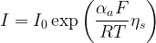
When the surface overpotential is large and anodic – that is, positive – the second term in the BV equation becomes negligible and we can make the approximation

$\displaystyle i\approx {{i}_{o}}\exp \left( {\frac{{{{\alpha }_{a}}F{{\eta }_{s}}}}{{RT}}} \right)$

This simplified expression is called the Tafel equation, named after the German scientist who discovered the relationship between the current equivalent to the rate of a single reaction on a metal surface and the potential of the metal. It can be readily solved for the overpotential as a function of current:

$\displaystyle i={{i}_{o}}\exp \left( {\frac{{{{\alpha }_{a}}F{{\eta }_{s}}}}{{RT}}} \right)\to \ln i=\ln {{i}_{o}}+\ln \left[ {\exp \left( {\frac{{{{\alpha }_{a}}F{{\eta }_{s}}}}{{RT}}} \right)} \right]$

$\displaystyle \therefore \ln i=\ln {{i}_{o}}+\frac{{{{\alpha }_{a}}F{{\eta }_{s}}}}{{RT}}$

$\displaystyle \therefore \frac{{RT}}{{{{\alpha }_{a}}F}}\ln i=\frac{{RT}}{{{{\alpha }_{a}}F}}\ln {{i}_{o}}+{{\eta }_{s}}$

$\displaystyle \therefore {{\eta }_{s}}=\frac{{RT}}{{{{\alpha }_{a}}F}}\ln i-\frac{{RT}}{{{{\alpha }_{a}}F}}\ln {{i}_{o}}$

This equation indicates that a plot of $\displaystyle {{\eta }_{s}}$ versus ln i should yield a straight line. Both the transfer coefficient $\displaystyle {{\alpha }_{a}}$ and the exchange current $\displaystyle {{i}_{o}}$ can be determined from such a plot. For good measurements, the fit should encompass at least one order of magnitude in current, preferably more.

In a similar manner, when the overpotential is large and cathodic – i.e., negative – it is the first term in the BV equation that becomes negligible, leading to the approximation

$\displaystyle i\approx {{i}_{o}}\exp \left( {-\frac{{{{\alpha }_{c}}F{{\eta }_{s}}}}{{RT}}} \right)$

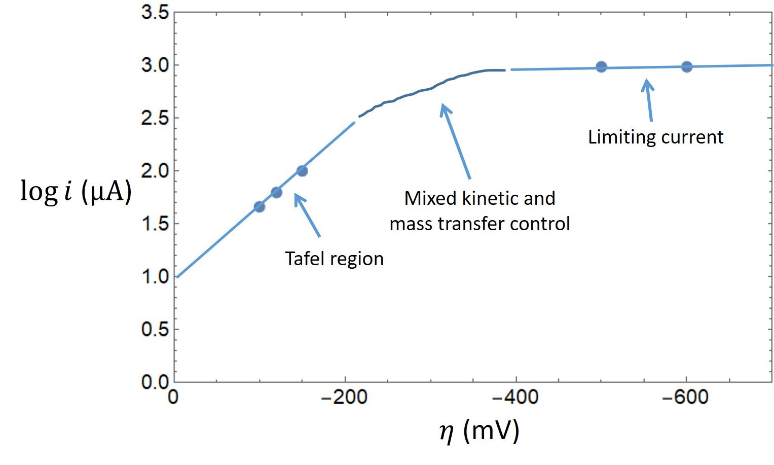
The utility of the Tafel equation depends on the relative magnitude of the overpotential applied to the system. When overpotentials are small (i.e., lower than 50 mV or so), the slope of the log i-overpotential curve increases because the backward electrochemical reaction becomes greater than 1% of the forward reaction, changing the relative concentrations at the electrode surface.

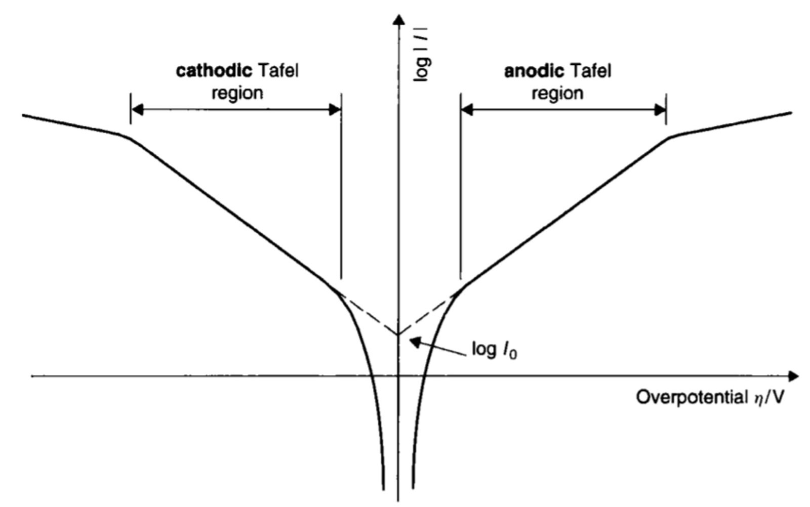
When overpotentials are large (i.e., greater than a few hundred mV), the log i-overpotential plot is linear and essentially horizontal, indicating that i is independent of overpotential. Here, the rate of mass transport is too small to bring sufficient material to the electrode/solution interface, thus signifying that the same amount of analyte is reduced (left-hand curve in Figure 1) or oxidized (right-hand curve) whatever the value of $\displaystyle \eta$ . We say that these horizontal wings of current-voltage plots represent the regions of mass transport control.

At intermediate overpotentials – by intermediate we mean absolute values of $\displaystyle \eta$ in the range of 100 mV to 300 mV or so – the logarithm of current becomes proportional to the overpotential and Tafel kinetics apply. This is the so-called Tafel region. In this segment of the graph, the slope of the line can be used to calculate the transfer coefficient, and the exchange current can be determined by extrapolating the line to its point of intersection with the vertical axis.

Much of electrochemical kinetics data, especially older data, were computed with base-10 logarithms. Accordingly, switching from natural logarithms to base-10 logarithms requires the inclusion of a factor ln 10 = 2.3. Applying this modification, the Tafel equation becomes

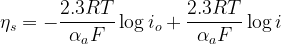
$\displaystyle {{\eta }_{s}}=-\frac{{2.3RT}}{{{{\alpha }_{a}}F}}\log {{i}_{o}}+\frac{{2.3RT}}{{{{\alpha }_{a}}F}}\log i$

or simply

$\displaystyle {{\eta }_{s}}=a+b\log i$

where

$\displaystyle a=-\frac{{2.3RT}}{{{{\alpha }_{a}}F}}\log {{i}_{o}}\,\,\,;\,\,\,b=\frac{{2.3RT}}{{{{\alpha }_{a}}F}}$

Figure 1. Schematic plot of log i against overpotential $\displaystyle \eta$ . The linear regions yield the Tafel slopes, from which the transfer coefficients $\displaystyle \alpha$ can be determined. The intersection between the two Tafel regions occurs at the y-axis at log $\displaystyle {{i}_{0}}$ .

An electrochemical current-potential plot can reveal more than just transfer coefficient and exchange current. Some other parameters that may be extracted from such a plot are briefly introduced below.

Standard rate constant. This parameter, $\displaystyle {{k}_{0}}$ , is a measure of the kinetic facility of a redox couple. A system with a large $\displaystyle {{k}_{0}}$ will achieve equilibrium on a short time scale, whereas a system with small $\displaystyle {{k}_{0}}$ will be sluggish. For a one-step, one-electron process in which the equilibrium concentrations of oxidant and reductant are the same, c, the standard rate constant is given by

$\displaystyle {{k}^{0}}=\frac{{{{i}_{0}}}}{{FAc}}$

Clearly, $\displaystyle {{k}^{0}}$ is proportional to exchange current and can often be used instead of $\displaystyle {{i}_{0}}$ in kinetic equations.

Charge transfer resistance. This parameter is the negative reciprocal slope of the current-potential curve where that curve passes through the origin. It is given by

$\displaystyle {{R}_{{ct}}}=\frac{{RT}}{{F{{i}_{0}}}}$

The charge transfer resistance serves as a measure of kinetic facility, and approaches zero for very large $\displaystyle {{k}_{0}}$ .

Mass transfer coefficient. This parameter, which should be familiar to students of convective mass transfer, measures the intensity of mass exchange at the electrode surface. It is related to the limiting current by the expression

$\displaystyle {{h}_{m}}=\frac{{{{i}_{L}}}}{{nFA{{h}_{m}}c*}}$

where $\displaystyle c*$ is the concentration of species in the bulk solution. Bear in mind that $\displaystyle {{h}_{m}}$ has units of length/time and is usually stated in cm/s.

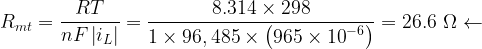
Mass transfer resistance. This parameter is interpreted as a resistance to mass transfer at low overpotentials, and can be expressed as

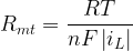
$\displaystyle {{R}_{{mt}}}=\frac{{RT}}{{nF\left| {{{i}_{L}}} \right|}}$

where n is the number of electrons transferred in the reaction.

A simple example (modified from Fuller & Harb, 2018)

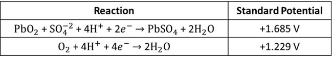
The evolution of oxygen is an important process in a lead-acid battery. Assume that the positive electrode of the flooded lead-acid battery is at its standard overpotential. Calculate the overpotential for the oxygen evolution reaction. It is reported that the Tafel slope for this reaction is 150 mV/decade at 25ºC. What is the transfer coefficient, $\displaystyle {{\alpha }_{a}}$ ? If the current exchange density is $\displaystyle 9.2\times {{10}^{{-7}}}$ A/m², what is the current density for oxygen evolution?

Given the Tafel slope = 0.15 V/decade, we can easily determine the transfer coefficient:

$\displaystyle \frac{{2.3RT}}{{{{\alpha }_{a}}F}}=0.15\to \alpha =\frac{{2.3RT}}{{0.15F}}$

$\displaystyle \therefore \alpha =\frac{{2.3\times 8.314\times 298}}{{0.15\times 96,485}}=0.394\leftarrow$

Now, the overpotential for this reaction is $\displaystyle {{\eta }_{s}}$ = 1.685 – 1.229 = 0.456 V. The current exchange density was given as $\displaystyle {{I}_{0}}$ = $\displaystyle 7.2\times {{10}^{{-7}}}$ A/m² (we are using a capital I to distinguish current density from current). Substituting in the Tafel equation, the current density for oxygen evolution is calculated to be

$\displaystyle I={{I}_{0}}\exp \left( {\frac{{{{\alpha }_{a}}F}}{{RT}}{{\eta }_{s}}} \right)$

$\displaystyle \therefore I=\left( {9.2\times {{{10}}^{{-7}}}} \right)\times \exp \left( {\frac{{0.394\times 96,485}}{{8.314\times 298}}\times 0.456} \right)=1.01\,\,\text{mA/}{{\text{m}}^{2}}\leftarrow$

An advanced example (modified from Bard & Faulkner, 2001)

The following data were obtained for the reduction of species $\displaystyle R$ to $\displaystyle {{R}^{-}}$ in a stirred solution at a 0.1-cm² electrode. The solution contained 0.01 M $\displaystyle {{R}^{-}}$ and 0.01 M $\displaystyle R$ . Experiments were conducted at a temperature of 25ºC.

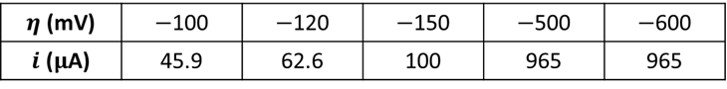
Determine the transfer coefficient, the exchange current, the standard rate constant, the charge transfer coefficient, the mass transfer coefficient, and the mass transfer resistance.

The tabulated data show that a limiting cathodic current of 965 $\displaystyle \mu$ A is reached at $\displaystyle \eta$ = -500 mV and -600 mV. Comparatively large overpotentials are required to enforce this current; hence, Tafel behavior should be observed for currents less than approximately 10% of the limiting current. A plot of the data is shown below.

The first three points outline a Tafel region with slope -6.77, from which we can easily determine the transfer coefficient:

$\displaystyle -6.77=-\frac{{\alpha F}}{{2.3RT}}\to \alpha =6.77\times \frac{{2.3RT}}{F}$

$\displaystyle \therefore \alpha =\frac{{6.77\times 2.3\times 8.314\times 298}}{{96,485}}=0.40\leftarrow$

Extrapolating the Tafel region of the plot to $\displaystyle \eta$ = 0 gives $\displaystyle {{\log }_{{10}}}{{i}_{0}}$ = 1.0, so that the exchange current is determined to be $\displaystyle {{i}_{0}}$ = 10 $\displaystyle \mu$ A.

Having obtained the exchange current, $\displaystyle {{k}_{0}}$ easily follows:

$\displaystyle {{i}_{0}}={{k}^{0}}FAc\to {{k}^{0}}=\frac{{{{i}_{0}}}}{{FAc}}$

$\displaystyle \therefore {{k}^{0}}=\frac{{10\times {{{10}}^{{-6}}}}}{{96,485\times 0.1\times \left( {0.01\times {{{10}}^{{-3}}}} \right)}}=1.04\times {{10}^{{-4}}}\,\text{cm/s}\leftarrow$

Likewise for $\displaystyle {{R}_{{ct}}}$ :

$\displaystyle {{R}_{{ct}}}=\frac{{RT}}{{F{{i}_{0}}}}=\frac{{8.314\times 298}}{{96,485\times \left( {10\times {{{10}}^{{-6}}}} \right)}}=2.57\,\,\text{k}\Omega \leftarrow$

The mass transfer coefficient is determined next:

$\displaystyle {{i}_{L}}={{h}_{m}}FAc\to {{h}_{m}}=\frac{{{{i}_{L}}}}{{FAc}}$

$\displaystyle \therefore {{h}_{m}}=\frac{{{{i}_{L}}}}{{FAc}}=\frac{{965\times {{{10}}^{{-6}}}}}{{96,485\times 0.1\times \left( {0.01\times {{{10}}^{{-3}}}} \right)}}=0.01\,\,\text{cm/s}\leftarrow$

Lastly, we compute the mass transfer resistance:

$\displaystyle {{R}_{{mt}}}=\frac{{RT}}{{nF\left| {{{i}_{L}}} \right|}}=\frac{{8.314\times 298}}{{1\times 96,485\times \left( {965\times {{{10}}^{{-6}}}} \right)}}=26.6\,\,\Omega \leftarrow$

References

• BARD, A. and FAULKNER, L. (2001). Electrochemical Methods: Fundamentals and Applications. Hoboken: John Wiley and Sons.

• FULLER, T. and HARB, J. (2018). Electrochemical Engineering. Hoboken: John Wiley and Sons.

• MONK, P. (2001). Fundamentals of Electroanalytical Chemistry. Hoboken: John Wiley and Sons.

Electrode Kinetics and the Tafel Equation

Subscribe to our Mailing List!

Featured Posts

A Primer on NAND Flash Memories

Solidification Time and Chvorinov’s Rule

Step-Growth Polymerization, the Carothers Equation, and the Flory-Schulz Distribution

More Articles

Tokamaks and the Grad-Shafranov Equation

Step-Growth Polymerization, the Carothers Equation, and the Flory-Schulz Distribution

Fields of Study

More

© 2024 Montogue Quiz

Subscribe to
our Mailing List!

Subscribe to our Mailing List!

Subscribe to receive our latest materials in your inbox.

Homework Help

© 2024 Montogue Quiz

Subscribe to our Mailing List!