Surface Chemistry, the Gibbs Adsorption Equation, and Adsorption Isotherms

In this article, we provide a quick introduction to adsorption science isotherms. We begin with a derivation of the Gibbs adsorption equation. Then, we introduce two of the most common adsorption isotherm models: the Langmuir isotherm and the BET isotherm. Each section is accompanied by an example problem.

1. The Gibbs adsorption equation (Shaw, 1992; Pashley & Karaman, 2004; Cosgrove, 2005)

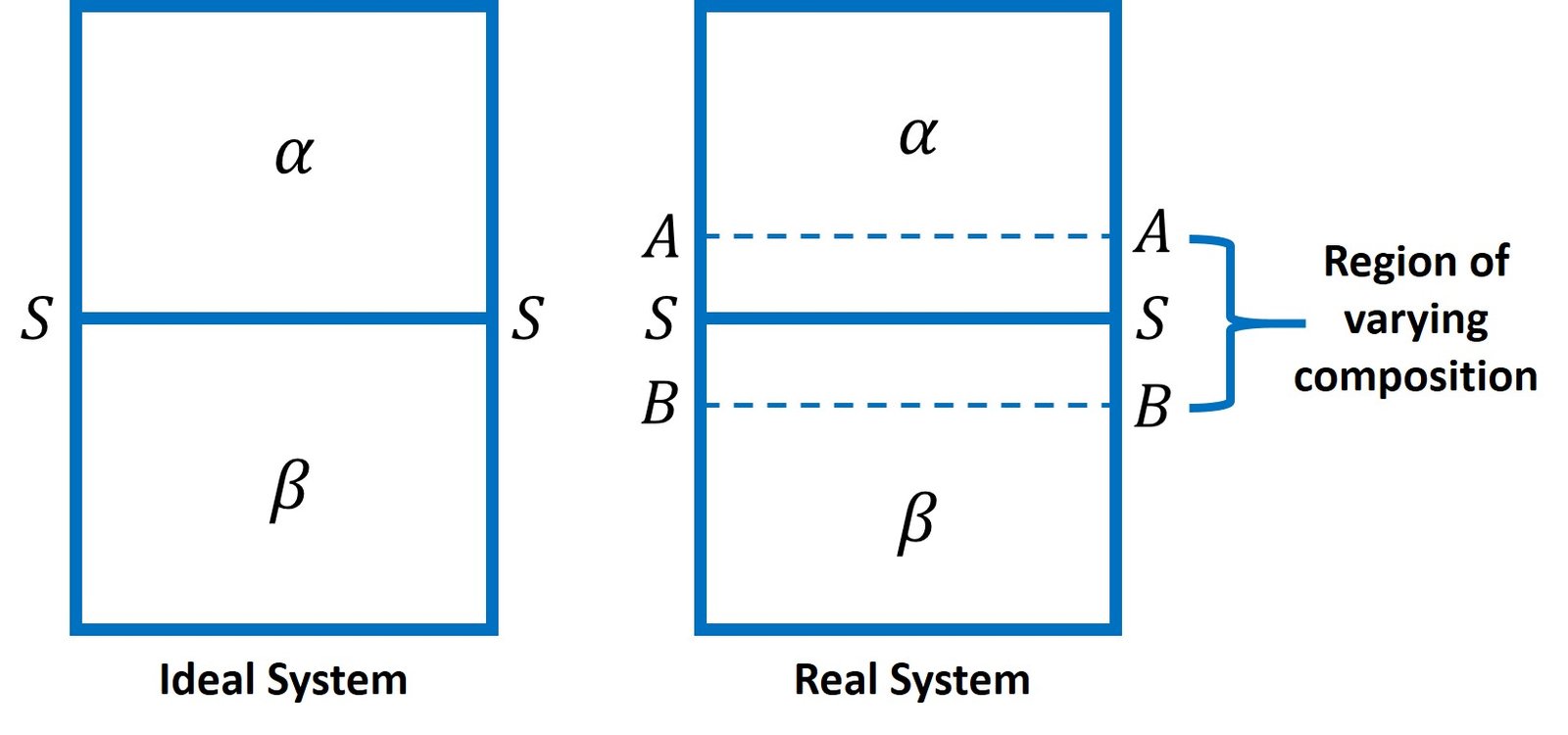
The Gibbs adsorption equation enables the extent of adsorption at a liquid surface to be estimated from surface tension data. Before deriving this expression, it is important to realize the limitations associated with this model – and, for that matter, all of the adsorption isotherms studied in this article. It is convenient to regard the interface between two phases as a mathematical plane, such as SS in Figure 1. This approach, however, is unrealistic, especially if an adsorbed film is present. Not only will such a film have a certain thickness, but also its presence may influence the nearby structure (for example, by dipole-dipole interaction, especially in an aqueous phase) and result in an interfacial region of varying composition with an appreciable thickness in terms of molecular dimensions. Nevertheless, theories based on discrete layer separation offer a good degree of accuracy relatively to experimental measurements. One of the earliest such models, proposed by the legendary American thermodynamicist, Josiah Gibbs, is briefly described below.

Figure 1. Interfaces in ideal and real systems.

If a mathematical plane is indeed taken to represent the interface between the two phases, adsorption can be described conveniently in terms of surface excess concentrations. Let us consider the interface between two phases, say between a liquid and a vapor, where a solute (i) is dissolved in the liquid phase. When the solute increases in concentration near the interface between the two phases, there must be a surface excess of solute $\displaystyle n_{i}^{\sigma }$ , compared with the bulk value continued right up to the interface. We can define a surface excess concentration, in moles per unit area, as

$\displaystyle {{\Gamma }_{i}}=\frac{{n_{i}^{\sigma }}}{A}$

where A is interfacial area. Bear in mind that $\displaystyle {{\Gamma }_{i}}$ may be positive or negative, and its magnitude depends on the location of SS, which is chosen somewhat arbitrarily as discussed above.

Let us now examine the effect of adsorption on the interfacial energy ( $\displaystyle \gamma$ ). If a solute i is positively adsorbed with a surface density of $\displaystyle {{\Gamma }_{i}}$ , we would expect the surface energy to decrease on increasing the bulk concentration of this component (and vice versa). This situation is illustrated in Figure 2, where the total free energy of the system $\displaystyle {{G}^{T}}$ and $\displaystyle {{\mu }_{i}}$ are both increased by addition of component i, but, because this component is favorably adsorbed at the surface (only relative to the solvent) since both have a higher energy state at the surface, the work required to create a new surface (i.e., $\displaystyle \gamma$ ) is reduced. Thus, although the total free energy of the system increases with the creation of new surface, this process is made easier as the chemical potential of the selectively adsorbed component increases (i.e., with concentration). This reduction in surface energy must be directly related to the change in chemical potential of the solute and to the amount adsorbed, and is therefore given by the simple relationship

$\displaystyle d\gamma =-{{\Gamma }_{i}}d{{\mu }_{i}}$

or, in the case of several components,

$\displaystyle d\gamma =-\Sigma \left( {{{\Gamma }_{i}}d{{\mu }_{i}}} \right)$

The change in $\displaystyle {{\mu }_{i}}$ is caused by the change in bulk solute concentration. The result above is the Gibbs surface tension equation. Basically, this equation describes the fact that increasing the chemical potential of the adsorbing species reduces the energy required to produce new surface (i.e., $\displaystyle \gamma$ ). This is the main physicochemical feature of surface-active materials, more commonly known as surfactants.

Figure 2. Change in surface energy caused by addition of a solute.

Gibbs’ equation can be readily extended to a solution of two components, in which case we may write

$\displaystyle d\gamma =-{{\Gamma }_{1}}d{{\mu }_{1}}-{{\Gamma }_{2}}d{{\mu }_{2}}$

and hence the adsorption excess for one of the components is given by

$\displaystyle {{\Gamma }_{1}}={{\left( {\frac{{\partial \gamma }}{{\partial {{\mu }_{1}}}}} \right)}_{{T,{{\mu }_{2}}}}}$

Thus, in principle, we could determine the adsorption excess of one of the components from surface tension measurements, if we could vary $\displaystyle {{\mu }_{1}}$ independently of $\displaystyle {{\mu }_{2}}$ . But this appears to not be possible, because the chemical potentials are dependent on the concentration of each component. However, for dilute solutions the change in $\displaystyle \mu$ for the solvent is negligible compared to that of the solute. Hence, the change for the solvent can be ignored, leading to the straightforward result

$\displaystyle d\gamma =-{{\Gamma }_{1}}d{{\mu }_{1}}$

Now, since

$\displaystyle {{\mu }_{1}}=\mu _{1}^{0}+RT\ln {{c}_{1}}$

differentiation with respect to concentration $\displaystyle {{c}_{1}}$ gives

$\displaystyle {{\left( {\frac{{\partial {{\mu }_{1}}}}{{\partial {{c}_{1}}}}} \right)}_{T}}=RT{{\left( {\frac{{\partial \ln {{c}_{1}}}}{{\partial {{c}_{1}}}}} \right)}_{T}}=\frac{{RT}}{{{{c}_{1}}}}$

so that, combining this result with the expression for $\displaystyle d\gamma$ , we ultimately obtain

$\displaystyle {{\Gamma }_{1}}=-\frac{1}{{RT}}{{\left( {\frac{{\partial \gamma }}{{\partial \ln {{c}_{1}}}}} \right)}_{T}}=-\frac{{{{c}_{1}}}}{{RT}}{{\left( {\frac{{\partial \gamma }}{{\partial {{c}_{1}}}}} \right)}_{T}}$

This relation is the Gibbs adsorption isotherm in its usual formulation. Experimental measurements of $\displaystyle \gamma$ over a range of concentrations allows us to plot $\displaystyle \gamma$ against $\displaystyle \ln {{c}_{1}}$ and thereby obtain $\displaystyle {{\Gamma }_{1}}$ , the adsorption density at the surface. The validity of this fundamental representation of adsorption phenomena has been corroborated by comparison with direct adsorption measurements.

It is important to bear in mind that the Gibbs equation in the form above applies to non-dissociating materials (e.g., non-ionic surfactants). For ionic surfactants of the form $\displaystyle {{R}^{-}}{{M}^{+}}$ , we can write, assuming ideal behavior,

$\displaystyle d\gamma =-{{\Gamma }_{R}}d{{\mu }_{R}}-{{\Gamma }_{M}}d{{\mu }_{M}}$

If no electrolyte is added, electroneutrality of the surface requires that $\displaystyle {{\Gamma }_{R}}$ = $\displaystyle {{\Gamma }_{M}}$ = $\displaystyle {{\Gamma }_{1}}$ . Substituting above brings to

$\displaystyle {{\Gamma }_{1}}=-\frac{1}{{2RT}}{{\left( {\frac{{\partial \gamma }}{{\partial \ln {{c}_{1}}}}} \right)}_{T}}$

Cosgrove (2005) recommends using the equation above with the mean ionic activity $\displaystyle {{a}_{1}}$ = $\displaystyle {{({{a}_{R}}{{a}_{M}})}^{{{1}/{2}\;}}}$ .

Example 1

For a $\displaystyle 1\times {{10}^{{-4}}}$ M aqueous solution of n-butanoic acid, $\displaystyle {{d\gamma }}/{{dc}}\;$ = –0.08 N-m²/mol at 25ºC. Using the Gibbs adsorption equation, determine the surface excess of butanoic acid and calculate the surface area available to each molecule.

Note that $\displaystyle 1.0\times {{10}^{{-4}}}$ mol/dm³ = 0.1 mol/m³. Substituting in the Gibbs equation gives

$\displaystyle {{\Gamma }_{1}}=-\frac{c}{{RT}}\frac{{d\gamma }}{{dc}}=-\frac{{0.1}}{{8.314\times 298}}\times \left( {-0.08} \right)=3.23\times {{10}^{{-6}}}\,\text{mol/}{{\text{m}}^{2}}\leftarrow$

The surface area available for each molecule is then

$\displaystyle {{a}_{m}}=\frac{1}{{\left( {3.23\times {{{10}}^{{-6}}}} \right)\times \left( {6.02\times {{{10}}^{{23}}}} \right)}}=5.14\times {{10}^{{-19}}}\,{{\text{m}}^{2}}=0.514\,\ \text{n}{{\text{m}}^{2}}\leftarrow$

2. Adsorption isotherms – the Langmuir isotherm (Modified from Tien, 2019)

The Langmuir isotherm is perhaps the most widely used isotherm expression for representing physical adsorption equilibrium data. Although it may be derived in several different ways, the kinetic approach is used in most textbooks. The basic assumptions are:

1. Adsorption of adsorbates takes place at well-defined sites.

2. All adsorption sites are the same (energetically), and each site accommodates only one adsorbate molecule.

3. There is no lateral interaction between adsorbed molecules.

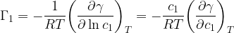
The adsorption rate is assumed to be

$\displaystyle \text{Adsorption rate}={{k}_{a}}P\left( {{{q}_{m}}-q} \right)$

where $\displaystyle {{k}_{a}}$ is the adsorption rate constant, $\displaystyle q$ is adsorption, $\displaystyle {{q}_{m}}$ is the maximum adsorption (when all sites are filled), and $\displaystyle P$ is the adsorbate pressure. The desorption rate, in turn, is given by

$\displaystyle \text{Desorption rate}={{k}_{d}}q$

where $\displaystyle {{k}_{d}}$ is the desorption rate constant. At equilibrium, we must have

$\displaystyle {{k}_{a}}P\left( {{{q}_{m}}-q} \right)={{k}_{d}}q$

$\displaystyle \therefore {{k}_{a}}P{{q}_{m}}-{{k}_{a}}Pq={{k}_{d}}q$

$\displaystyle \therefore {{k}_{a}}P{{q}_{m}}=({{k}_{d}}+{{k}_{a}}P)q$

$\displaystyle \therefore \frac{{{{k}_{a}}P{{q}_{m}}}}{{{{k}_{d}}+{{k}_{a}}P}}=q$

$\displaystyle \therefore \frac{{{{k}_{a}}P}}{{{{k}_{d}}+{{k}_{a}}P}}=\frac{q}{{{{q}_{m}}}}$

Let $\displaystyle q$ / $\displaystyle {{q}_{m}}$ = $\displaystyle \theta$ and $\displaystyle {{k}_{a}}$ / $\displaystyle {{k}_{d}}$ = $\displaystyle K$ . The latter is the Langmuir adsorption constant. Making these substitutions brings to

$\displaystyle \frac{{{{k}_{a}}P}}{{{{k}_{d}}+{{k}_{a}}P}}=\frac{q}{{{{q}_{m}}}}\to \theta =\frac{{KP}}{{1+KP}}$

This is the basic form of the Langmuir adsorption isotherm.

Example 2

At 273 K and 10 bar, the Langmuir adsorption of a gas on a solid surface gave the fraction of surface coverage as 0.01. In this case, what is the value of the Langmuir adsorption constant?

From the Langmuir isotherm equation, we have

$\displaystyle \theta =\frac{{K{{P}_{A}}}}{{1+K{{P}_{A}}}}$

We were given the fraction of surface coverage $\displaystyle \theta$ = 0.01 and the pressure $\displaystyle {{P}_{A}}$ = 10 bar. Substituting and solving for K, it follows that

$\displaystyle \theta =\frac{{K{{P}_{A}}}}{{1+K{{P}_{A}}}}\to 0.01=\frac{{K\times 10}}{{1+K\times 10}}$

$\displaystyle 0.01+0.1K=10K$

$\displaystyle 0.01=9.9K$

$\displaystyle K=\frac{{0.01}}{{9.9}}=1.01\times {{10}^{{-3}}}\,\text{ba}{{\text{r}}^{{-1}}}\leftarrow$

3. Adsorption isotherms – the Brunauer-Emmet-Teller (BET) isotherm (Ghosh, 2009)

The theory of chemical adsorption proposed by Langmuir is based on the formation of a monolayer. However, multilayers can form in physical adsorption. The isotherm in the case of a monolayer assumes the shape shown as Type I in Figure 3. The extent of adsorption increases with pressure and ultimately reaches a limiting value, as predicted by the Langmuir theory. However, for adsorption involving multilayer formation at low temperatures, at least four other types of adsorption isotherm can be observed; see below. (In the graphs shown, y denotes the amount of gas adsorbed by m kg of adsorbent at pressure P.)

Figure 3. Adsorption isotherms.

To explain such varied adsorption isotherms, Brunauer, Emmet and Teller proposed, in 1938, a theory of multilayer adsorption. They posited that, even after the formation of the monolayer, other layers of gas may condense on it. Langmuir’s idea of fixed adsorption sites was, however, retained. They suggested that there is equilibrium between the first layer and the adsorbent, and similar dynamic criteria were assumed to exist for the successive molecular layers. The Van der Waals forces provide the binding energy in these successive layers. The equation derived by them is

$\displaystyle \frac{P}{{V\left( {{{P}^{{\text{sat}}}}-P} \right)}}=\frac{1}{{{{V}_{m}}C}}+\frac{P}{{{{P}^{{\text{sat}}}}}}\left( {\frac{{C-1}}{{{{V}_{m}}C}}} \right)$

where $\displaystyle V$ is the volume of gas adsorbed under a pressure $\displaystyle P$ , $\displaystyle {{P}^{{\text{sat}}}}$ is the saturated vapor pressure, $\displaystyle {{V}_{m}}$ is the volume of gas adsorbed when the surface is covered with a monolayer, and $\displaystyle C$ is a constant that can be related to the heat of adsorption of the first layer ( $\displaystyle {{E}_{1}}$ ) and the enthalpy of liquefaction of the gas ( $\displaystyle {{E}_{L}}$ ),

$\displaystyle C=\exp \left( {\frac{{{{E}_{1}}-{{E}_{L}}}}{{RT}}} \right)$

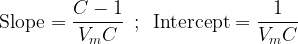
From the BET equation, it is clear that a plot of $\displaystyle P/V({{P}^{{sat}}}-P)$ versus $\displaystyle P/{{P}^{{\text{sat}}}}$ should yield a straight line with the following characteristics:

$\displaystyle \text{Slope}=\frac{{C-1}}{{{{V}_{m}}C}}\,\,\,;\,\,\,\text{Intercept}=\frac{1}{{{{V}_{m}}C}}$

Accordingly, $\displaystyle {{V}_{m}}$ can be determined with the simple relation

$\displaystyle {{V}_{m}}=\frac{1}{{\text{Slope}+\text{Intercept}}}$

Thus, the BET equation permits us to extract from multilayer adsorption data the volume of adsorbed gas that would saturate the surface if the adsorption were limited to a monolayer. The most immediate application of this quantity is the calculation of specific surface area. The volume of gas adsorbed when the surface is covered by a monolayer, $\displaystyle {{V}_{m}}$ , is recorded at standard temperature and pressure, STP, at which the volume occupied by one mole of gas is $\displaystyle 22.4\times {{10}^{{-3}}}$ m³. The number of moles of gas adsorbed is $\displaystyle {{N}_{A}}{{V}_{m}}$ /( $\displaystyle 22.4\times {{10}^{{-3}}}$ ), where $\displaystyle {{N}_{A}}$ is Avogadro’s number. If the cross-section of each adsorbed gas molecule is $\displaystyle \sigma$ and if m kg of adsorbent is present, then the surface area per kg of adsorbent is given by

$\displaystyle {{S}_{{sp}}}=\frac{{{{N}_{A}}{{V}_{m}}\sigma }}{{m\times 22.4\times {{{10}}^{{-3}}}}}$

Here, $\displaystyle {{V}_{m}}$ is expressed in m³ and $\displaystyle \sigma$ in m². The following example illustrates use of the BET isotherm in calculations of specific surface area.

Example 3

The following data were obtained for adsorption of nitrogen on 0.88 kg of nitrogen-activated alumina. The data are adapted from Tien (2019).

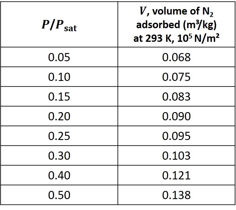
A) Estimate the volume of nitrogen adsorbed over 1 kg of alumina when a monolayer is formed.

B) Calculate the specific surface area of this alumina sample. The area occupied by one nitrogen molecule is $\displaystyle 16\times {{10}^{{-20}}}$ m².

According to the BET model, a plot of $\displaystyle {{\left( {{P}/{{{{P}_{{\text{sat}}}}}}\;} \right)}}/{{V\left( {1-{P}/{{{{P}_{{\text{sat}}}}}}\;} \right)}}\;$ versus $\displaystyle P/{{P}_{{\text{sat}}}}$ should yield a straight line. The data we need are processed below.

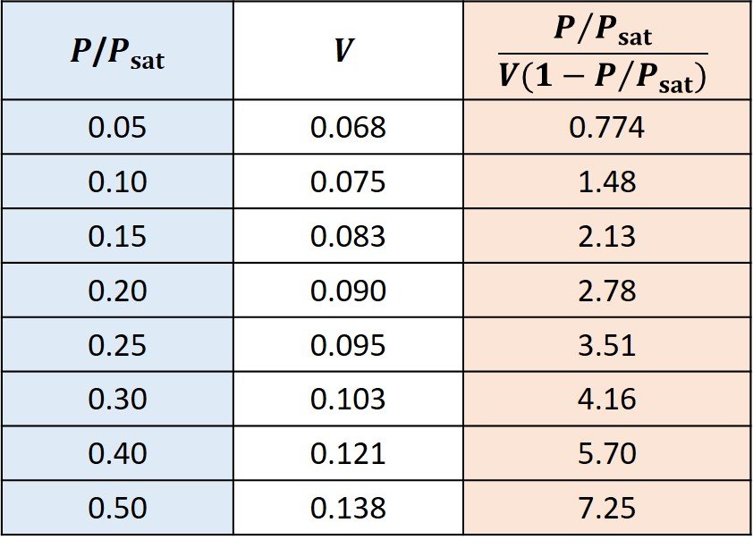
Then, the data in the red column are plotted against the data in the blue column, as shown.

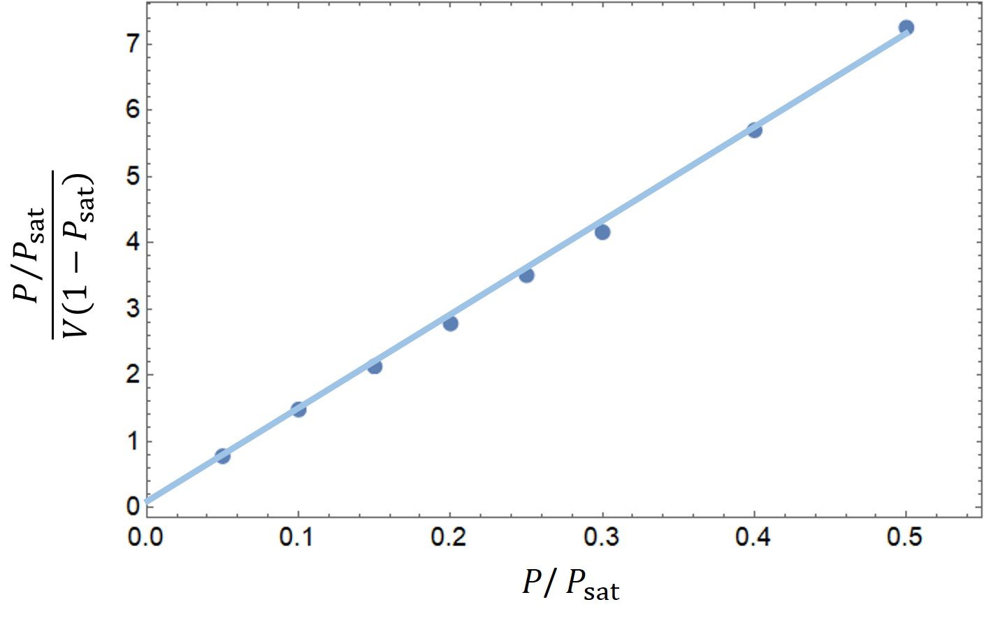
Clearly, there is a linear trend in this dataset. Fitting these data to a first-degree equation yields a line with slope

$\displaystyle \text{Slope}=\frac{{C-1}}{{{{V}_{m}}C}}=13.4$

and intercept

$\displaystyle \text{Intercept}=\frac{1}{{{{V}_{m}}C}}=0.125$

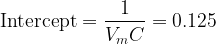
Solving both equations simultaneously gives $\displaystyle {{V}_{m}}$ = 0.0739 m³ and $\displaystyle C$ = 108.2. The volume of nitrogen adsorbed over 1 kg of alumina is then

$\displaystyle V=\frac{{0.0739}}{{0.88}}=0.0840\,\,{{\text{m}}^{3}}\,\,\text{for }m=1\,\,\text{kg }\leftarrow$

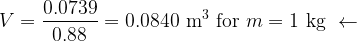
Lastly, the specific surface area is

$\displaystyle {{A}_{{sp}}}=\frac{{{{N}_{A}}{{V}_{m}}\sigma }}{{m\times 22.4\times {{{10}}^{{-3}}}}}=\frac{{\left( {6.02\times {{{10}}^{{23}}}} \right)\times 0.0739\times \left( {16\times {{{10}}^{{-20}}}} \right)}}{{0.88\times \left( {22.4\times {{{10}}^{{-3}}}} \right)}}=361,000\,\,{{{{\text{m}}^{2}}}}/{{\text{kg}}}\;\leftarrow$

References

• COSGROVE, T. (Ed.) (2005). Colloid Science: Principles, Methods and Applications. Oxford: Blackwell Publishing.

• GHOSH, P. (2009). Colloid and Surface Science. New Delhi: PHI Learning.

• PASHLEY, R. and KARAMAN, M. (2004). Applied Colloid and Surface Chemistry. Hoboken: John Wiley and Sons.

• SHAW, D. (1992). Introduction to Colloid and Surface Chemistry. 4th edition. Oxford: Butterworth-Heinemann.

• TIEN, C. (2019). Introduction to Adsorption. Amsterdam: Elsevier.

Surface Chemistry, the Gibbs Adsorption Equation, and Adsorption Isotherms

Subscribe to our Mailing List!

Featured Posts

A Primer on NAND Flash Memories

Solidification Time and Chvorinov’s Rule

Step-Growth Polymerization, the Carothers Equation, and the Flory-Schulz Distribution

More Articles

Aldohexoses: Classification, Haworth Projections, and Chair Conformations

Electrode Kinetics and the Tafel Equation

Fields of Study

More

© 2024 Montogue Quiz

Subscribe to
our Mailing List!

Subscribe to our Mailing List!

Subscribe to receive our latest materials in your inbox.

Homework Help

© 2024 Montogue Quiz

Subscribe to our Mailing List!