Four Models for One-Dimensional Infiltration of Water in Soils

In this article, we discuss four simple mathematical equations used to model one-dimensional infiltration of water in soils.

1. Generalities

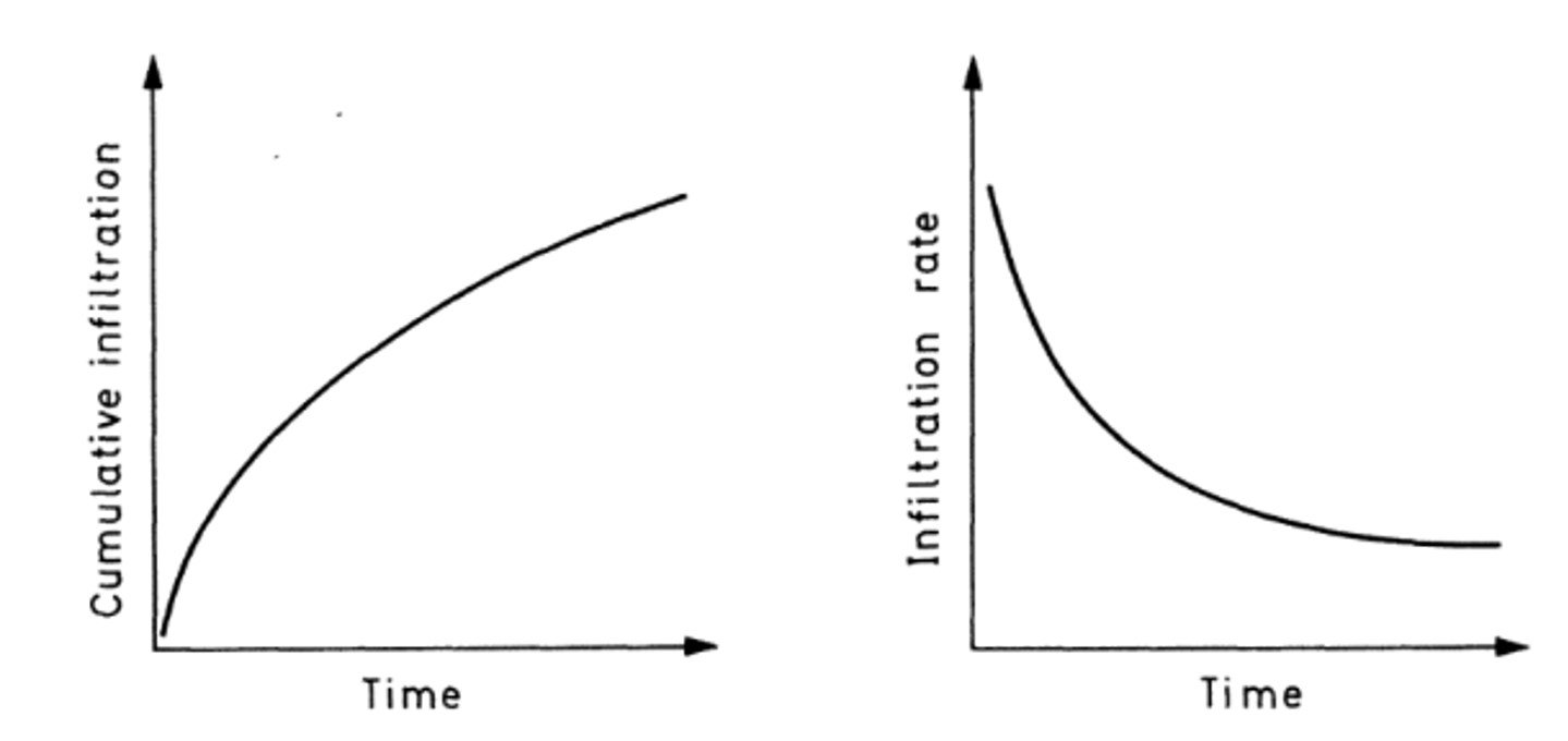
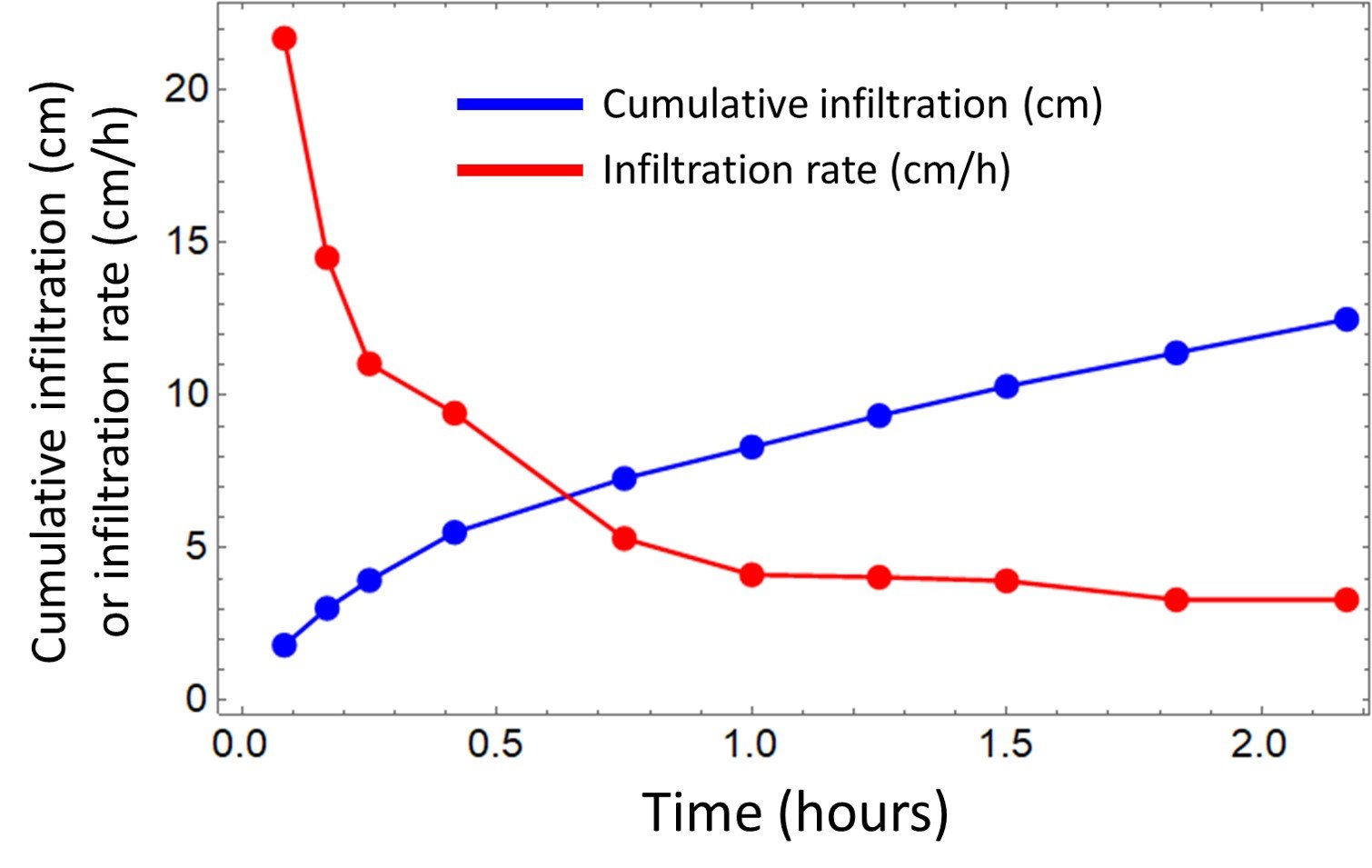
Before anything else, we should get acquainted with two concepts: cumulative infiltration and infiltration rate. Cumulative infiltration is the total volume of water infiltrated per unit area of soil surface during a specified time period; it is expressed in units of length. Infiltration rate, in turn, is the time derivative of cumulative infiltration. A graph of cumulative infiltration as a function of time is shown in Figure 1. The amount of water infiltrating the soil increases rather rapidly (the curve has a steep slope) at the beginning of infiltration; as time increases, the cumulative infiltration increases more slowly (the curve has a much smaller slope). Infiltration rate as a function of time is also graphed on Figure 1. Its value is high at the beginning of infiltration; as time increases, however, the wetting front continuously progresses along the soil column and water is transmitted to the wetting front through a wet zone that is continuously increasing in length. This increases the resistance to flow and decreases the infiltration rate. The trends illustrated in Figure 1 apply to most soils, but not to swelling soils.

Figure 1. Cumulative infiltration and infiltration rate.

Several models of one-dimensional infiltration of water in soils have been developed in the 20th century. Four of them are discussed in this article: the Lewis-Kostiakov equation, the Horton equation, the Green-Ampt equation, and the Philip equation.

2. The Lewis-Kostiakov equation

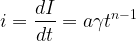
The Lewis equation was developed in the 1926 by Mortimer Reed Lewis, an irrigation engineer at Oregon State College. Some authors unduly attribute it to A. Kostiakov, a Russian soil scientist who proposed a similar result in the 1930s. Lewis’s result is a simple exponential law,

$\displaystyle I=\gamma {{t}^{a}}$

where I is the cumulative infiltration between time zero and t, and $\displaystyle \gamma$ and a are constants. Constant $\displaystyle \gamma$ is positive, while a ranges from zero to unity. Deriving the equation above with respect to time gives the infiltration rate,

$\displaystyle i=\frac{{dI}}{{dt}}=a\gamma {{t}^{{n-1}}}$

The Lewis equation is empirical in nature and has no physical basis. Nevertheless, exponential relations such as the one associated with this model are simple to use and often cover a wide range of time values with decent accuracy.

3. The Horton equation

The Horton equation was developed by Robert E. Horton, a pioneer of field studies on infiltration, during the 1930s. His result is

$\displaystyle i={{i}_{f}}+\left( {{{i}_{0}}-{{i}_{f}}} \right)\exp \left( {-\beta t} \right)$

where i₀ is the initial infiltration rate, i_f is the final infiltration rate achieved at large times – sometimes known as the constant rate or the ultimate infiltration capacity – and $\displaystyle \beta$ is a soil parameter that describes the rate of decrease of infiltration. Horton felt that the reduction in infiltration rate with time was largely controlled by factors operating at the soil surface. These included swelling of soil colloids and the closing of small cracks, which progressively sealed the soil surface. He also recognized that a bare soil surface was compacted by raindrops, but crop cover mitigated their effect. Horton’s field data showed that the infiltration rate eventually approached a constant value, which was often somewhat smaller than the saturated permeability of the soil. The latter observation was thought to be due to air entrapment.

Although not steeped in theoretical concepts as the Green-Ampt and Philip equations (see below), the Horton equation has become one of the most widely used soil infiltration equations. It is the equation of choice in many hydrology codes developed in the 1970s and 1980s, including the popular EPA Storm Water Management Model (SWMM). Comparative investigations carried out between the late 1960s and the 1980s revealed that the Horton equation indeed provides consistently more accurate results than the theoretical models in a number of situations. However, researchers note that, like other empirical models, the calibrated coefficient values of Horton’s equation are fitted parameters with no physical meaning and apply only to the field condition in which they were determined.

Example 1

Infiltration capacity data obtained in a flooding type infiltration test is given below.

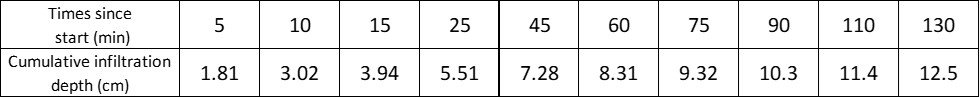
Plot the cumulative infiltrations and the infiltration rates as functions of time. Then, determine the initial infiltration rate i₀, the ultimate infiltration capacity i_f, and the decay parameter $\displaystyle \beta$ in Horton’s model.

The data are processed below.

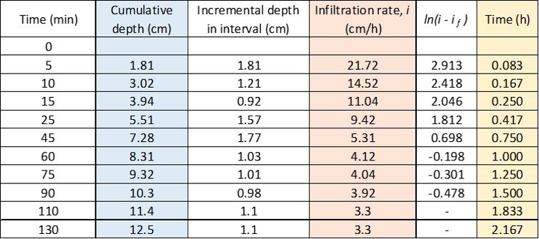
Then, the cumulative infiltrations (blue column above) and infiltration rates (red column) are plotted as functions of time (yellow column).

In order to determine the parameters of the Horton model, we appeal to the corresponding equation and apply logarithms to both sides, giving

$\displaystyle i={{i}_{f}}+\left( {{{i}_{0}}-{{i}_{f}}} \right)\exp \left( {-\beta t} \right)$

$\displaystyle \therefore i-{{i}_{f}}=\left( {{{i}_{0}}-{{i}_{f}}} \right)\exp \left( {-\beta t} \right)$

$\displaystyle \therefore \ln \left( {i-{{i}_{f}}} \right)=\ln \left[ {\left( {{{i}_{0}}-{{i}_{f}}} \right)\exp \left( {-\beta t} \right)} \right]$

$\displaystyle \therefore \ln \left( {i-{{i}_{f}}} \right)=\ln \left( {{{i}_{0}}-{{i}_{f}}} \right)-\beta t$

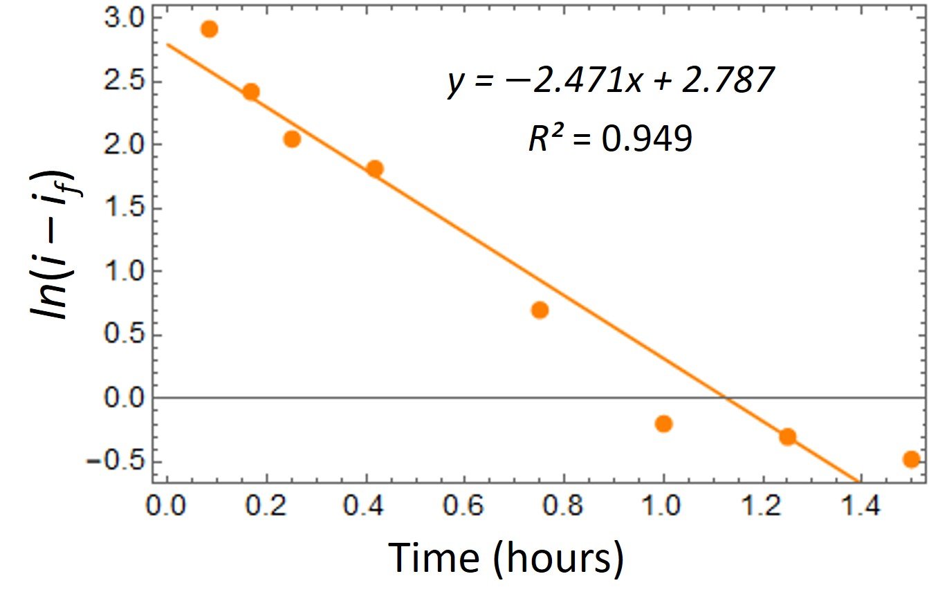
Clearly, a plot of ln(i – i_f) versus time should yield a straight line with slope $\displaystyle -\beta$ and intercept ln(i₀ – i_f). The logarithms we need were computed in the second-to-last column of the previous table. These data are plotted against time in the following graph.

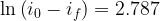
From the slope of the line, we see that $\displaystyle \beta$ = 2.471 h^-1. From the intercept with the y-axis, in turn, we have

$\displaystyle \ln \left( {{{i}_{0}}-{{i}_{f}}} \right)=2.787$

Inspecting the red column of the foregoing table, we read i_f = 3.3 cm/h. It remains to compute i₀,

$\displaystyle \ln \left( {{{i}_{0}}-3.3} \right)=2.787\to {{i}_{0}}=19.53\,\,\text{cm/h}$

Finally, the Horton equation that models infiltration in this soil is

$\displaystyle i={{i}_{f}}+\left( {{{i}_{0}}-{{i}_{f}}} \right)\exp \left( {-\beta t} \right)$

$\displaystyle \therefore i=3.3+\left( {19.53-3.3} \right)\exp \left( {-2.471t} \right)$

$\displaystyle \therefore i=3.3+16.23\exp \left( {-2.471t} \right)\leftarrow$

4. The Green-Ampt equation

In 1911, W. Heber Green and G.A. Ampt in Australia published an infiltration model based on a simple physical model of soil. Infiltrated water is assumed to move downward through the soil with an abrupt wetting front separating the wetted and unwetted zones. At any instant the potential infiltration rate, i_p, is given by the equation

$\displaystyle {{i}_{p}}=K\left[ {1+\frac{{{{\Psi }_{f}}\left( {\phi -{{\theta }_{i}}} \right)}}{I}} \right]$

where K is the hydraulic conductivity of the transmission zone, $\displaystyle {{\Psi }_{f}}$ is the capillary suction head at the wetting front, $\displaystyle \phi$ is the porosity of the soil (the volumetric water content at saturation), $\displaystyle {{\theta }_{i}}$ is the initial volumetric water content of the soil, and I is cumulative infiltration. The time required for a soil to achieve a cumulative infiltration I is given by

$\displaystyle t={{t}_{p}}+\frac{1}{{{{K}_{s}}}}\left\{ {I-{{I}_{p}}+{{\Psi }_{f}}\left( {\phi -{{\theta }_{i}}} \right)\ln \left[ {\frac{{{{\Psi }_{f}}\left( {\phi -{{\theta }_{i}}} \right)+{{I}_{p}}}}{{{{\Psi }_{f}}\left( {\phi -{{\theta }_{i}}} \right)+I}}} \right]} \right\}$

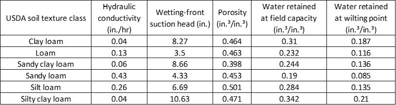
where t_p is the time at the onset of ponding, I_p is the cumulative infiltration at time t_p, and I is the cumulative infiltration at time t. Table 1 lists some values of the parameters used in the Green-Ampt equation based on some 5000 soil horizons compiled by the US Agricultural Research Service in the 1980s. Bear in mind that the data are in USCS units.

Table 1. Physical properties of loam soils

Example 2

A 45-minute rainfall with a constant intensity of 4 cm/hr occurs on a typical silt-loam soil that is initially at field capacity. Determine the time to the onset of ponding and the cumulative infiltration.

With reference to Table 1, the values of the Green-Ampt parameters are K = 0.26 $\displaystyle \times$ 2.54 = 0.660 cm/hr, $\displaystyle {{\Psi }_{f}}$ = 6.69 $\displaystyle \times$ 2.54 = 17.0 cm, $\displaystyle \phi$ = 0.501, and $\displaystyle {{\theta }_{i}}$ = 0.284 (since the soil is initially at field capacity). The cumulative infiltration at the onset of ponding, I_p, is found by setting the potential infiltration rate equal to the rainfall rate and solving for I. In the case at hand,

$\displaystyle {{i}_{p}}=K\left[ {1+\frac{{{{\Psi }_{f}}\left( {\phi -{{\theta }_{i}}} \right)}}{{{{I}_{p}}}}} \right]\to 4=0.660\times \left[ {1+\frac{{17.0\times \left( {0.501-0.284} \right)}}{{{{I}_{p}}}}} \right]$

$\displaystyle \therefore {{I}_{p}}=0.716\,\,\text{cm}$

Accordingly, ponding begins when approximately 0.72 cm of infiltration has occurred. Until ponding begins, the actual infiltration rate equals the rainfall rate, so the time to the onset of ponding, t_p, is 0.716/4 = 0.179 h, or 10.7 minutes. The cumulative infiltration at any time during ponding can be established by taking the second Green-Ampt equation, setting t equal to 45 min = 0.75 h, and solving for I,

$0.75=0.179+\frac{1}{{0.66}}\left\{ {I-0.716+17.0\times \left( {0.501-0.284} \right)\times \log \left[ {\frac{{17.0\times \left( {0.501-0.284} \right)+0.716}}{{17.0\times \left( {0.501-0.284} \right)+I}}} \right]} \right\}$

One way to solve this equation is by dint of Mathematica’s Solve command,

This returns a meaningless negative solution and I = 2.10 cm, which is the cumulative infiltration we seek. Neglecting rainfall interception and other abstractions, we could just as well compute the total runoff, which is given by the difference between the rainfall, 0.75 $\displaystyle \times$ 4 = 3 cm, and the cumulative infiltration I = 2.10 cm; that is,

$\displaystyle \text{Runoff}=3.0-2.1=0.9\,\,\text{cm}$

5. The Philip equation

The Philip two-term infiltration equation, first published by J. Philip in 1957, is a truncated form of a physically based converging series solution that desribes cumulative infiltration under ponded conditions. The equation has the form

$\displaystyle I=S{{t}^{{{1}/{2}\;}}}+At$

where t is time, S is sorptivity, and A is an empirical constant with units of length over time. Sorptivity is a measure of the soil to absorb water. It is numerically equal to the cumulative infiltration during the first unit of time. For initially dry soils (initial volume water content $\displaystyle {{\theta }_{i}}$ = 0), its value varies from about 5 $\displaystyle \times$ 10^-5 m/s^1/2 (0.04 cm/min^1/2) for a heavy clay soil to about 2 $\displaystyle \times$ 10^-3 m/s^1/2 (1.5 cm/min^1/2) for a coarse sand. The second coefficient of interest in the equation, A, is related to the hydraulic conductivity of the soil. Indeed, when considering infiltration over a relatively long period of time, some researchers have suggested that the saturated hydraulic conductivity can be readily substituted for A. In spite of its convenience, researchers have indicated that this approximation may lead to overprediction of cumulative infiltration with increasing time.

The first term on the right-hand side of the Philip equation gives the gravity-free absorption into a ponded soil due to capillary and adsorption. The second term represents the ability of the soil to transmit water under the influence of gravity in the transition zone. The first term dominates the infiltration process during the early water transport stage. In this interval, the gravitational component, represented by the second term in the equation, is so small that the infiltration proceeds at almost the same rate as it would if infiltration were horizontal. As infiltration continues, the second term becomes gradually more important until it dominates the infiltration process. These features of the Philip model are illustrated in the following example.

Example 3

In a horizontal infiltration run for a permeable sandy soil, the initial and saturated volumetric water contents were established as $\displaystyle {{\theta }_{{vi}}}$ = 0.15 and $\displaystyle {{\theta }_{{vs}}}$ = 0.60, respectively, and a sharp wetting front had progressed 10 cm from the source in 16 min. The saturated hydraulic conductivity of the soil was 0.02 cm/min. Plot the vertical and horizontal infiltrations for 1, 10, 100, 1000, 10,000, and 100,000 min.

Where there is a sharp wetting front, the sorptivity can be estimated as

$\displaystyle S=\frac{{\left( {{{\theta }_{{vs}}}-{{\theta }_{{vi}}}} \right)h}}{{{{t}^{{{1}/{2}\;}}}}}=\frac{{\left( {0.60-0.15} \right)\times 10}}{{{{{16}}^{{{1}/{2}\;}}}}}=1.13\,\,\text{cm/mi}{{\text{n}}^{{{1}/{2}\;}}}$

Coefficient A can be equated to the hydraulic conductivity = 0.02 cm/min. We can then determine the cumulative infiltrations from the Philip equation. As an example, for t = 10 min,

$\displaystyle S{{t}^{{{1}/{2}\;}}}=1.13\times {{10}^{{0.5}}}=3.57\,\,\text{cm}$

$\displaystyle At=0.02\times 10=0.2\,\,\text{cm}$

so that the horizontal infiltration is determined to be

$\displaystyle {{I}_{x}}=S{{t}^{{{1}/{2}\;}}}=3.57\,\text{cm}$

while the vertical infiltration is calculated to be

$\displaystyle {{I}_{y}}=S{{t}^{{{1}/{2}\;}}}+At=3.57+0.2=3.77\,\text{cm}$

Infiltrations for other time values are tabulated below.

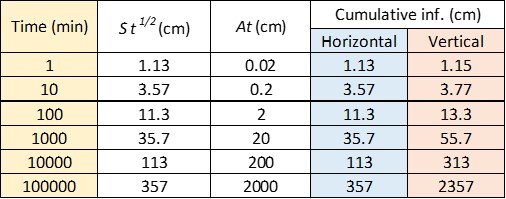
The data in question are plotted below. For convenience, we choose a bilogarithmic plot.

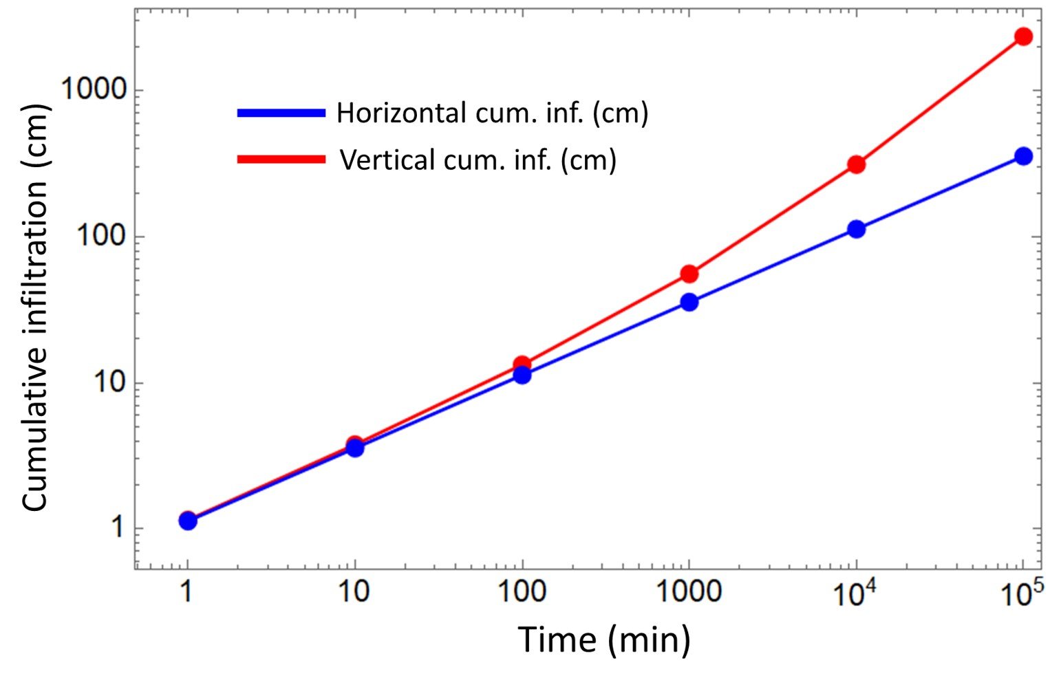
As evidenced by these curves, at short times the vertical and horizontal infiltrations are very similar; but at longer times, the vertical infiltration greatly exceeds the horizontal. For vertical flow, the St^1/2 term is dominant at short times, but at 10⁵ min, At has come to dominance.

Go further

More problems on soil infiltration for agriculture and earth science students can be found in our free soil physics and chemistry quiz, which you can find here. Civil engineering students will surely appreciate our closely related quiz on flow of water through soil.

References

• King, R. (1992) Overview and Bibliography of Methods for Evaluating the Surface-Water Infiltration Component of the Rainfall-Runoff Process. Reston: US Geological Survey.

• KIRKHAM, M. (2005). Principles of Soil and Plant Water Relations. Amsterdam: Elsevier.

• KOOREVAAR, P., MENELIK, G., and DIRKSEN, C. (1983). Elements of Soil Physics. Amsterdam: Elsevier.

• MIYAZAKI, T. (2006). Water Flow in Soils. 2nd edition. Boca Raton: CRC Press.

• SUBRAMANYA, K. (2008). Engineering Hydrology. 3rd edition. New Delhi: Tata McGraw-Hill.

Four Models for One-Dimensional Infiltration of Water in Soils

Subscribe to our Mailing List!

Featured Posts

A Primer on NAND Flash Memories

Solidification Time and Chvorinov’s Rule

Step-Growth Polymerization, the Carothers Equation, and the Flory-Schulz Distribution

More Articles

River Meandering Models

The Bruun Rule and Sea-Level Rise

Fields of Study

More

© 2024 Montogue Quiz

Subscribe to
our Mailing List!

Subscribe to our Mailing List!

Subscribe to receive our latest materials in your inbox.

Homework Help

© 2024 Montogue Quiz

Subscribe to our Mailing List!