
1. Introduction to saltwater intrusion in coastal aquifers
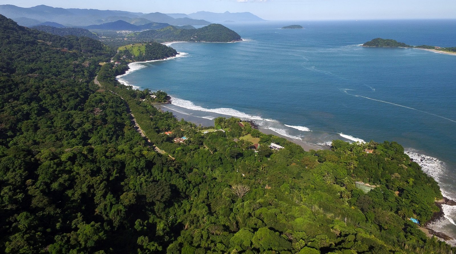
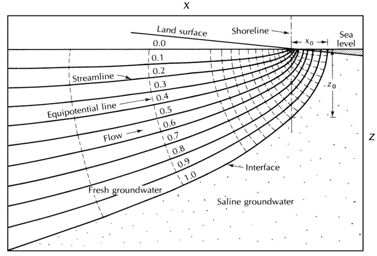
Coastal aquifers constitute an important source for water, especially in arid and semi-arid zones which border the sea. Many coastal areas are also heavily urbanized, a fact which makes the need for freshwater even more acute. Figure 1 gives a typical cross-section of a coastal phreatic aquifer with exploitation. It can be seen that there exists a body of seawater, in the form of a wedge, underlying the freshwater. As in the case of most illustrations describing flow in aquifers, these are highly distorted figures, not drawn to scale.
Figure 1. Illustration of saltwater intrusion in a coastal aquifer.
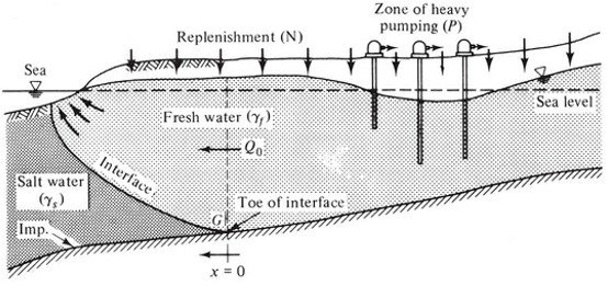
Under natural undisturbed conditions in a coastal aquifer, a state of equilibrium is maintained, with a stationary interface and a freshwater flow to the sea above it. At every point on this interface, the elevation and the slope are determined by the freshwater potential and gradient (or flow velocity). The continuous change of slope results from the fact that as the sea is approached, the specific discharge of freshwater tangent to the interface increases. By pumping from a coastal aquifer in excess of replenishment, the water table (or the piezometric surface) in the vicinity of the coast is lowered to the extent that the piezometric head in the freshwater body becomes less than in the adjacent seawater wedge, and the interface starts to advance inland until a new equilibrium is reached. This phenomenon is called seawater intrusion or encroachment. Seawater encroachment can be passive, passive-active, or active. These occur, respectively, when fresh groundwater flows only towards the sea, flows both inland and towards the sea, and flows inland only. The salient features of each type are listed in Table 1 and illustrated in Figure 2.
Table 1. Types of saltwater intrusion. Detailed explanations of each type can be found in Werner (2016).
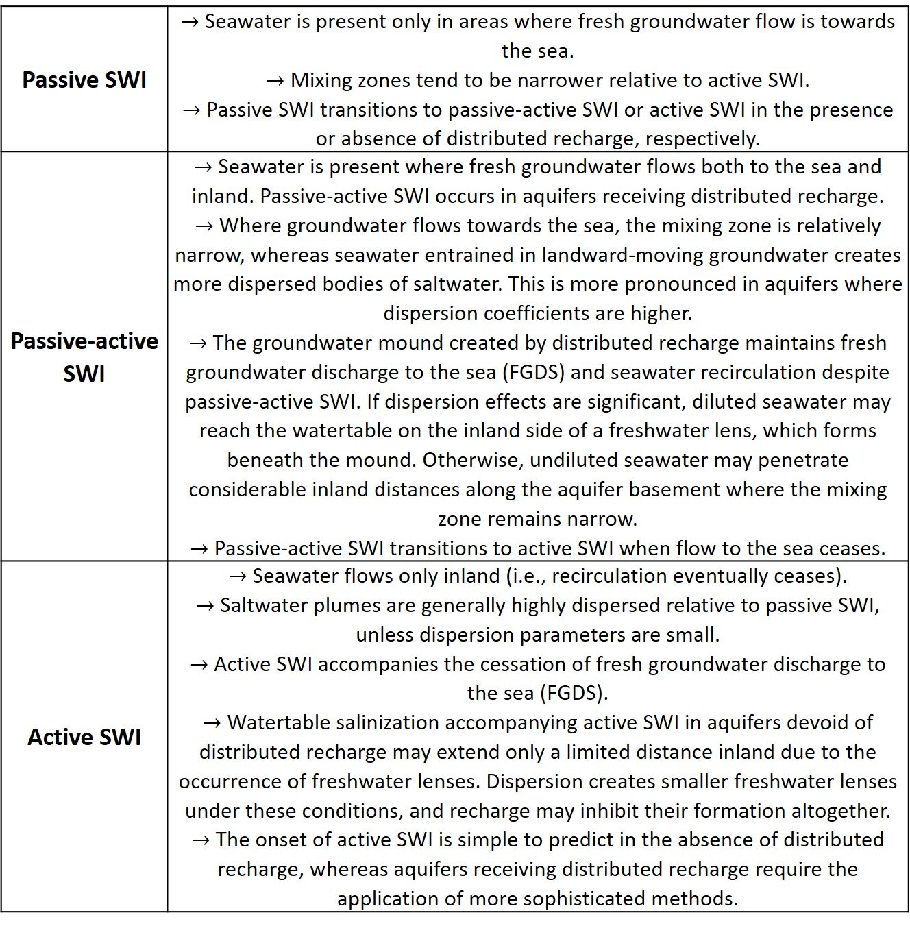
Figure 2. SWI occurring under three alternative freshwater flow situations: (a) seaward freshwater flow (causing passive SWI); (b) both seaward and landward freshwater flow (causing passive SWI); and (c) landward freshwater flow (causing active SWI). Dashed lines represent steady-state conditions prior to SWI. Sharp-interface representations of the mixing zone are used for ease of illustration. From Werner (2016).
The primary detrimental effects of seawater intrusion are reduction in the available freshwater storage volume and contamination of production wells. Salinization of water supplies has been associated with a number of negative effects. For one, use of saline water in soil irrigation hinders the development of plants and ultimately reduces agricultural output (Shrivastava and Kumar, 2015). Further, human consumption of saline water has been linked to a greater risk of cardiovascular disease (Vineis et al., 2011). Also, the corrosivity of water increases proportionally to salinity for salt levels up to 3% (Kirk and Pikul, 1990).
Seawater intrusion involves mixing between saline and freshwater components. Because of its significant salt content, a small fraction of seawater would dominate the chemical composition of the groundwater mixture. Contribution of 1% of seawater would almost triple the salinity of typical groundwater (with an initial chloride content of 100 mg/L). Contribution of 5% of seawater would result in water with a salinity above 1000 mg/L.
Saltwater intrusion affects drinking water quality and, as in the case of other hydrologic pollution phenomena, calls for some quantitative measurement of practical interest. With this goal in mind, Tomaszkiewicz et al. (2014) proposed a seawater intrusion groundwater quality index, GQISWI, which ranges from 0 to 100, where 0 is indicative of seawater and 100 represents freshwater. The score is made up of two independent components: the freshwater-seawater index GQIPiper(mix) and the seawater fraction index GQIfsea, which are combined in the simple equation

The first component, GQIPiper(mix), is a score extracted from a modified version of the hydrochemical pattern diagram due to Piper (1944). The second component, GQIfsea, is dependent on the salt concentration of the groundwater sample. Tomaszkiewicz et al. (2014) argued that the two contributions to GQISWI had important limitations when used alone; for example, GQIfsea fails to recognize most hydrogeochemical reactions associated with seawater intrusion, such as cation exchanges, which may have a greater effect on the composition of aquifers subject to SWI than the Cl– concentrations upon which the GQIfsea is based. Thus, an arithmetic mean such as (I) seemed a straightforward approach to minimize limitations of each component.
Saltwater encroachment inland is the most important source of salinity increase in costal groundwater, but other sources and processes can contribute expressively to this phenomenon (Custodio, 1997). Examples include entrapped fossil seawater in unflushed parts of the aquifer following invasion of seawater during relatively high sea levels; sea-spray accumulation; evaporite rock dissolution; and pollution from sources such as sewage effluents, industrial effluents, mine water, road de-icing salts, and effluents from water softening or de-ionization plants. When the goal is the differential identification of the sources and dating of a saltwater intrusion episode, reliance on chemical tracers has proven useful. For example, Han et al. (2011), working in the Quaternary aquifer of Laizhou Bay, China, found that paleo-geological intrusion of brines with a TDS (total dissolved solids) > 100 g/L constituted the main source of salt in the brackish water moving towards the pumping wells in the area, rather than recently intruded seawater. Importantly, those authors noted, the origin of salinity in that aquifer is complex and could only be assessed by the simultaneous evaluation of several hydrochemical and isotopic parameters.
2. The mixing zone
In a SWI episode, the boundary between seawater and freshwater is known as the mixing or transition zone. In mathematical treatments of SWI, the mixing zone can be represented by a sharp interface between fresh and saline water. This simplification is convenient and makes the groundwater system amenable to simple analytical modelling techniques, but tends to oversimplify the real situation. In more realistic models, the sharp interface is replaced with a true diffuse interface in which there is a gradual variation in fluid density as the spatial domain extends from freshwater to seawater. Of course, modelling a density-dependent system is computationally expensive in view of the coupled, highly nonlinear nature of the flow and transport equations that accompany such a model. There are important advantages to these more advanced approaches, however; for one, only variable density models provide salinity predictions that can then be compared to field salinity measurements (Werner et al., 2012).
Observed mixing-zone thicknesses vary substantially between laboratory experiments, field situations and numerical simulations. Narrow mixing zones in homogeneous porous media were demonstrated in several laboratory experiments (e.g., Abarca and Clement, 2009). In contrast, mixing zones in field situations vary widely, ranging from meters to kilometers (see the review by Werner et al., 2012). The geomorphologic and geochemical composition of heterogeneous aquifers may also influence mixing-zone thicknesses, in addition to its important role in solute transport; for example, Oki et al. (1998), working in the coastal aquifer system of southern Oahu, Hawaii, found that stratigraphic variation was a strong control in mixing zone widths. The variability of possible geological structure combinations presents a significant barrier to the generalization of heterogeneity effects on saltwater intrusion phenomena.
It is also worth noting that the mixing zone is by no means a fixed space. Its shape and position are functions of the volume of fresh water discharging from the aquifer. Any action that changes the volume of freshwater discharge results in a consequent change in the saltwater-freshwater boundary. What’s more, minor fluctuations in the boundary position occur with tidal actions and seasonal and annual changes in the amount of freshwater discharge. For this reason, the transition zone is in a state of quasi-equilibrium (Fetter, 2014).
3. Mathematical modelling of SWI
Over a century ago, two groups of investigators, working independently along the European coast, proposed a simple model for static equilibrium in a coastal aquifer subjected to SWI. The Ghyben-Herzberg relation, as it is now known, gives the depth to which freshwater extends below sea level,
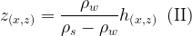
where 


That is, this result indicates that the depth to which freshwater extends below sea level is approximately 40 times the height of the water table above sea level.
Of course, the Ghyben-Herzberg relation is an oversimplification of the real freshwater-saltwater domain, in that it requires the two fluid regions to be static. Actual flow in a coastal aquifer can be modelled by combining the Ghyben-Herzberg relation with the Dupuit equations for one-dimensional flow. Such a model gives rise to the following equation for the x– and z– coordinates of the interface:

where 

The only difference between this equation and the previous one is that a constant has been added to the right-hand side. This ensures that z will still have a value at x = 0. Indeed, the depth (

In a similar manner, the width (
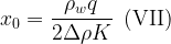
Figure 3. Glover’s (1964) profiles for saltwater intrusion.
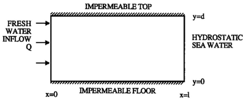
Other analytical and semianalytical solutions of interest in saltwater intrusion dynamics exist, and several have been compiled by Bruggeman (1999). Historically, the most important solution comes from the so-called Henry problem (Croucher and O’Sullivan, 1995), which is the only analytic solution for steady saltwater intrusion with variable density flow (Werner, 2012). In the Henry problem (Figure 4), a vertical slice is taken through a homogeneous isotropic aquifer confined above and below by impermeable boundaries. A constant flux of freshwater is applied to one end, while the other end is exposed to a stationary body of seawater. Saltwater intrudes from the seaward end until an equilibrium is reached with the opposing freshwater inflow. Since Harold Henry published his solution as a Ph.D. dissertation in 1964, the original problem has been reworked by several investigators in order to reconcile Henry’s analytical results with diverging numerical solutions. Along the way, some of the limitations of the problem were resolved, the most important being the fact that Henry’s original profiles are relatively insensitive to density-coupling effects – a crucial drawback if the Henry problem is to be employed as a benchmark for SWI codes. Simpson and Clement (2004) formulated and solved a new Henry problem to address the density-coupling sensitivity issue.
Figure 4. The Henry problem.
4. Recent topics: Bed slope, sea-level rise, Watson-Morgan overshoot
In the past 20 years, research on novel aspects of saltwater intrusion has produced some interesting insights. One topic that went largely unexplored until recently was the aquifer bed slope issue. Most coastal aquifers have inclined bed boundaries, but until recently models conceptualized geological formations with horizontal beds only. This is a mathematical convenience that may lead to inaccurate predictions. For example, Abarca (2007) formulated density-dependent flow processes in a three-dimensional confined aquifer geometry with allowance for a lateral slope of aquifer boundaries, and found that the intrusion of seawater was controlled more by the added slope than by aquifer thickness and dispersivity. Interest in sloped aquifer problems rekindled in recent years, as evidenced, e.g., by the work of Koussis et al. (2012), who developed a model to evaluate the impact of sea-level rise on seawater intrusion in both flux-controlled and head-controlled sloping unconfined coastal aquifers. Later, Mazi et al. (2013) employed the Koussis et al. (2012) model to investigate seawater intrusion in three major Mediterranean aquifers. More recently, another group (Lu et al., 2016) published its own analytical solutions for flow in sloping aquifers, including some of the first such results for seawater intrusion in confined sloping aquifers. Armanuos et. al (2020) conjugated the model of Lu et al. (2016) with a simulation on the use of barrier walls, one of the most reliable techniques for facilitating retreat of saltwater intrusion. They specified three values of sloping bed – one positive, one horizontal, and one negative – and verified that the slope of the aquifer is a vital parameter on determining the intrusion length in the sloping bed aquifer, compared with the horizontal one.
Another topic of growing interest is the impact of sea-level rise on saltwater intrusion, as pioneered by Sherif and Singh (1999) and Kooi et al. (2000). Saltwater intrusion is expected to worsen much sooner than other phenomena related to climate change-induced sea-level rise – one group aptly refers to it as the “leading edge of sea-level rise” (Tully et al., 2019) – and may affect ecological and human communities that have not experienced or adapted to salinity, leading to novel biogeochemical, ecological, and human land use transitions. Importantly, one group (Ferguson and Gleeson, 2012) has contended that coastal aquifers are more vulnerable to groundwater extraction than to predicted sea-level rise.
Papers on the relation between sea-level rise and saltwater intrusion are becoming more sophisticated by the year. To mention one important advancement, Abdouhalik and Ahmed (2018) replaced the assumption of an instantaneous sea-level rise – which may cause estimated SWI to be more rapid than would occur in gradual SLR (Ketabchi et al., 2016) – with an experimental method based on incremental steps on sea-level height. In doing so, Abdouhalik and Ahmed (2018) confirmed the intuitive predictions that a rising seawater level induced an increase in the supply of saline water into the aquifer model, whereas a drop in sea level was accompanied by a retreat of the saltwater wedge towards the coastline. Abdouhalik and Ahmed (2018) also found that the saltwater intrusion process caused by sea level changes induced faster and larger intrusion lengths than those caused by freshwater fluctuations, assuming the same absolute head change magnitude. Perhaps most interesting, however, is their finding that the receding rate of the saltwater wedge was relatively faster than the intruding rate, regardless of whether the incremental change was in the freshwater region or the seawater level; in one case, the intruding wedge required twice as long as the receding wedge to reach steady-state conditions.
Transient SLR-SWI studies such as that of Watson et al. (2010) have reported the occurrence of an overshoot phenomenon, whereby the freshwater-saltwater interface temporarily extends farther inland than the eventual post-sea-level rise steady state interface location. The saltwater intrusion overshoot phenomenon has potentially significant implications for coastal aquifer management, as it implies that the steady-state saltwater intrusion extent may not be the worst case, in contrast to what is generally assumed. Watson et al. (2010) hypothesized that overshoot is linked to the time required for the flow field to reequilibrate following seawater level retreat. The time for the flow field to reequilibrate is the time needed for head and flow to approach their final post-seawater level retreat steady state values. Heads and flows will change slightly thereafter due to changes in the position of the interface. Importantly, Watson et al. (2010) found the largest overshoot in cases where the characteristic time Tc for head response was large, where
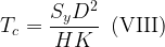
in which Sy is specific yield, D is domain length, H is aquifer thickness, and K is hydraulic conductivity. In a sand-tank simulation, Morgan et al. (2013) confirmed Watson’s intuition by showing that overshoot will be largest in systems where the head response time is large.
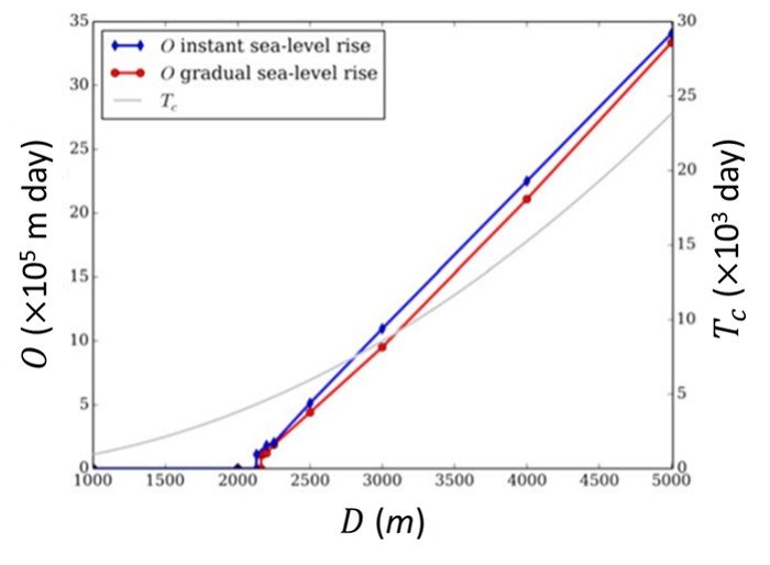
Studying the time scales of seawater intrusion and retreat, Lu and Werner (2013) did not observe Watson-Morgan overshoot when SWI was caused by a freshwater-level drop, but did notice a slight overshoot in their simulation of fast seawater retreat. Working with a numerical model, Morgan et al. (2015) showed that significant overshoot can occur under realistic unconfined aquifer settings for both instantaneous and gradual-sea-level rise scenarios. In their model, Morgan et al. (2015) saw that a relationship between overshoot and the K 
Figure 5. Relationship between integrated overshoot (O, m
References
Download references list here.