Drawdown in Aquifers: Theis and Hantush-Jacob Well Functions

In this post, we discuss two simple models for unsteady groundwater flow in aquifers. The first is the Theis model, which is used to assess the drawdown afforded by wells in confined aquifers. The second is the Hantush-Jacob model, which applies to leaky semiconfined aquifers. The MATLAB codes for example problems 1 to 3 can be downloaded in this Google Drive folder.

1. The Theis solution for wells in a confined aquifer

The confined-aquifer flow equation in radial coordinates can be expressed as (see Figure 1)

$\displaystyle \frac{{{{\partial }^{2}}s}}{{\partial {{r}^{2}}}}+\frac{1}{r}\frac{{\partial s}}{{\partial r}}=\frac{S}{T}\frac{{\partial s}}{{\partial t}}\,\,\,(1)$

where s(r,t) = h₀ – h is the drawdown, h₀ is the initial piezometric head, h is the piezometric head at a radial distance r from the well, t is time, S is the storativity (or storage coefficient) of the aquifer, and T is the transmissivity of the aquifer. In 1935, C.E. Theis published a solution to equation (1) based on an analogy with radial heat transfer. The Theis model is based on several assumptions, namely:

The aquifer is homogeneous and isotropic.
The aquifer is uniform in thickness and the pumping never affects its exterior boundary (i.e., the aquifer can be considered infinite in areal extent).
The aquifer is confined and does not receive any recharge.
Well discharge is derived entirely from aquifer storage.
The water removed from storage is discharged instantaneously when the head is lowered.
The pumping rate is constant.
The radius of the well is infinitely small, so that storage in the well can be ignored altogether.
The pumping well is fully penetrating, so it receives water from the entire thickness of the aquifer and it is 100% efficient (there are no well losses).
The initial potentiometric surface (before pumping) is horizontal.

Figure 1. A well in a confined aquifer.

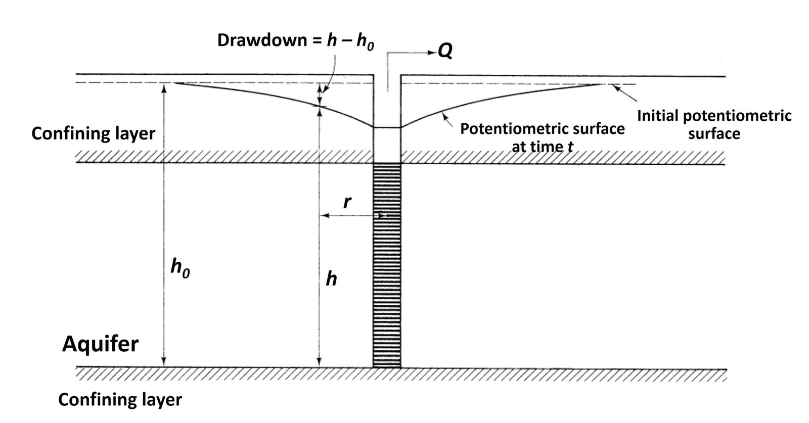
In his derivation, Theis worked with two boundary conditions. The first BC is that the potentiometric surface formed by the well is initially horizontal,

$\displaystyle s\left( {r,t=0} \right)=0\,\,\,\text{for all }r\,\,\,(2)$

The second BC relates to the assumption that the aquifer has an infinite horizontal extent and that there is no drawdown at very long distances from the well,

$\displaystyle s\left( {r\to \infty ,t} \right)=0\,\,\,\text{for all }t$

$\displaystyle \underset{{r\to 0}}{\mathop{{\lim }}}\,r\frac{{\partial s}}{{\partial r}}=-\frac{Q}{{2\pi T}}\,\,\,(3)$

where Q is the pumping rate in the well. Pressing on with his solution, Theis obtained the following expression for aquifer drawdown s,

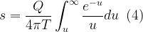
$\displaystyle s=\frac{Q}{{4\pi T}}\int_{u}^{\infty }{{\frac{{{{e}^{{-u}}}}}{u}du}}\,\,\,(4)$

where u is given by

$\displaystyle u=\frac{{{{r}^{2}}S}}{{4Tt}}\,\,\,(5)$

The integral in (4) is a modified version of the so-called exponential integral; it is a special function that appears in unsteady problems of fields such as heat transfer and neutron transport. In the mathematical literature, exponential integrals are written with the notations Ei(u) and E₁(u), but groundwater scientists traditionally adopt the notation W(u), so (4) can be restated as

$\displaystyle s=\frac{Q}{{4\pi T}}W\left( u \right)\,\,\,(6)$

Equation (6) can be used to compute the drawdown afforded by a well in a confined aquifer.

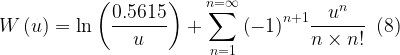
A note on the well function

The well function can be expressed by the series expansion

$\displaystyle W\left( u \right)=-0.5772-\ln u+u-\frac{{{{u}^{2}}}}{{2\times 2!}}+\frac{{{{u}^{3}}}}{{3\times 3!}}-\frac{{{{u}^{4}}}}{{4\times 4!}}+(...)\,\,\,(7)$

which has the general form

$\displaystyle W\left( u \right)=\ln \left( {\frac{{0.5615}}{u}} \right)+\sum\limits_{{n=1}}^{{n=\infty }}{{{{{\left( {-1} \right)}}^{{n+1}}}\frac{{{{u}^{n}}}}{{n\times n!}}}}\,\,\,(8)$

Example problem 1

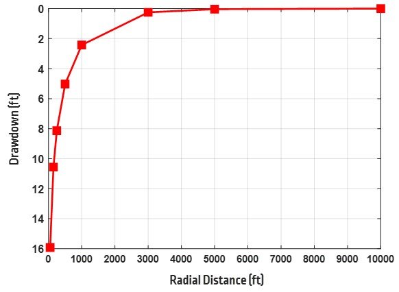
A well that is screened in a confined aquifer is to be pumped at a rate of 165,000 ft³/day for 30 days. If the aquifer transmissivity is 5320 ft²/day, and the storativity is 0.0007, what is the drawdown at distances of 50, 150, 250, 500, 1000, 3000, 5000, and 10,000 ft?

The solution to this problem is provided in code theis.m. As an example, we shall carry out the calculations for r = 500 ft. We first compute argument u,

$\displaystyle u=\frac{{{{r}^{2}}S}}{{4Tt}}=\frac{{{{{500}}^{2}}\times 0.0007}}{{4\times 5320\times 30}}=2.74\times {{10}^{{-4}}}$

The corresponding well function W(u) can be determined using MATLAB’s built-in function expint, which yields W(u) $\displaystyle \approx$ 7.63. We proceed to compute the drawdown s,

$\displaystyle s=\frac{Q}{{4\pi T}}W\left( u \right)=\frac{{165,000}}{{4\pi \times 5320}}\times 7.63=18.8\,\,\text{ft}$

Thus, after 30 days of pumping the drawdown at a distance of 500 ft from the well equals 18.8 ft. Similar calculations are carried out for other distances. The calculations are automated in theis.m. The drawdown-versus-distance plot is shown below.

2. Determining aquifer transmissivity and storativity with the Cooper-Jacob method

Importantly, the Theis solution is not just a tool for calculating well drawdowns; with the proper adjustments, it can also be used to determine the storativity and transmissivity of a confined aquifer. C.E. Jacob and H.H. Cooper observed that after a pumping well has been running for some time, u becomes small and the higher-power terms in the series expansion for well function W(u) (equation (7)) can be neglected with little loss of precision. Therefore, if

$\displaystyle \frac{{{{r}^{2}}S}}{{4Tt}}<0.05\,\,\,(9)$

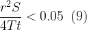
we can state that

$\displaystyle s\approx \frac{Q}{{4\pi T}}\left[ {-0.5772-\ln \left( u \right)} \right]$

$\displaystyle \therefore s=\frac{Q}{{4\pi T}}\left[ {-0.5772-\ln \left( {\frac{{{{r}^{2}}S}}{{4Tt}}} \right)} \right]$

$\displaystyle \therefore s=\frac{Q}{{4\pi T}}\left[ {-\ln \left( {1.78} \right)-\ln \left( {\frac{{{{r}^{2}}S}}{{4Tt}}} \right)} \right]$

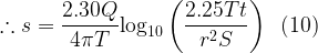
$\displaystyle \therefore s=\frac{Q}{{4\pi T}}\left[ {\ln \left( {\frac{{4Tt}}{{1.78\times {{r}^{2}}S}}} \right)} \right]$

$\displaystyle \therefore s=\frac{Q}{{4\pi T}}\ln \left( {\frac{{2.25Tt}}{{{{r}^{2}}S}}} \right)$

$\displaystyle \therefore s=\frac{{2.30Q}}{{4\pi T}}{{\log }_{{10}}}\left( {\frac{{2.25Tt}}{{{{r}^{2}}S}}} \right)\,\,\,(10)$

On semilog paper, equation (10) plots as a straight line if the limiting condition is met.

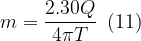
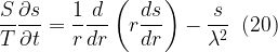
In a Cooper-Jacob drawdown-time analysis, drawdown measurements are made in an observation well at various times; distance r is therefore constant. A plot is made between drawdown, s (linear scale on vertical coordinate), and time, t (log scale on horizontal coordinate) (Figure 2a). With reference to equation (10), the slope of the line is

$\displaystyle m=\frac{{2.30Q}}{{4\pi T}}\,\,\,(11)$

$\displaystyle m=\frac{s}{{{{{\log }}_{{10}}}\left( {{{{{t}_{2}}}}/{{{{t}_{1}}}}\;} \right)}}=\frac{{2.30Q}}{{4\pi T}}\,\,\,(12)$

For a change in drawdown encompassing one log cycle, we have log(t₂/t₁) = 1 and equation (12) reduces to

$\displaystyle \frac{s}{{1.0}}=\frac{{2.30Q}}{{4\pi T}}$

$\displaystyle \therefore s=\frac{{2.30Q}}{{4\pi T}}\,\,\,(13)$

Solving for transmissivity,

$\displaystyle T=\frac{{2.30Q}}{{4\pi s}}\,\,\,(14)$

In turn, where the straight line intersects the x-axis, the drawdown is zero and the time is t₀. Substituting these values into (10), we have

$\displaystyle \therefore s=0=\frac{{2.30Q}}{{4\pi T}}{{\log }_{{10}}}\left( {\frac{{2.25T{{t}_{0}}}}{{{{r}^{2}}S}}} \right)$

$\displaystyle \therefore 0={{\log }_{{10}}}\left( {\frac{{2.25T{{t}_{0}}}}{{{{r}^{2}}S}}} \right)\,\,\,(15)$

Noting that 10⁰ = 1, we can remove the logarithm and solve for storativity,

$\displaystyle 1=\frac{{2.25T{{t}_{0}}}}{{{{r}^{2}}S}}$

$\displaystyle \therefore {{r}^{2}}S=2.25T{{t}_{0}}$

$\displaystyle \therefore S=\frac{{2.25T{{t}_{0}}}}{{{{r}^{2}}}}\,\,\,(16)$

To summarize, equations (14) and (16) can be used to yield the transmissivity and storativity of a confined aquifer, respectively.

Figure 2. Cooper-Jacob method. (a) Drawdown-time analysis. (b) Drawdown-distance analysis. (c) Drawdown-t²/r analysis.

It is important to note that at least two variants of the Cooper-Jacob technique have been used in groundwater practice. The first variant is a drawdown-distance analysis, whereby drawdown measurements are made at a given time in various wells, so it is time, not distance, that is held constant. A plot is made between drawdown s on the vertical scale and distance r on a logarithmic horizontal scale (Figure 2b). From similar considerations as in drawdown-time analysis, the transmissivity is given by

$\displaystyle T=\frac{{2.30Q}}{{2\pi s}}\,\,\,(17)$

and the storativity is

$\displaystyle S=\frac{{2.25Tt}}{{r_{0}^{2}}}\,\,\,(18)$

where r₀ is the intercept at the x-axis. The second – and most general – variant is to obtain measurements from several wells at various times and plot drawdown versus log₁₀(t/r²) as shown in Figure 2c. Then, the transmissivity has the same form as equations (14) and (17), whereas the storativity is expressed as

$\displaystyle S=2.25T{{\left( {\frac{t}{{{{r}^{2}}}}} \right)}_{0}}\,\,\,(19)$

where (t/r²)₀ is the intercept of the straight line on the x-axis.

Example problem 2

The following data are taken from a pumping test wherein a well was pumped at a rate of 0.45 cubic feet per second. The drawdown data is for an observation well located 240 ft away from the pumped well. Plot the data on semilogarithmic paper and use the Cooper-Jacob method to estimate the transmissivity and storativity of the local aquifer.

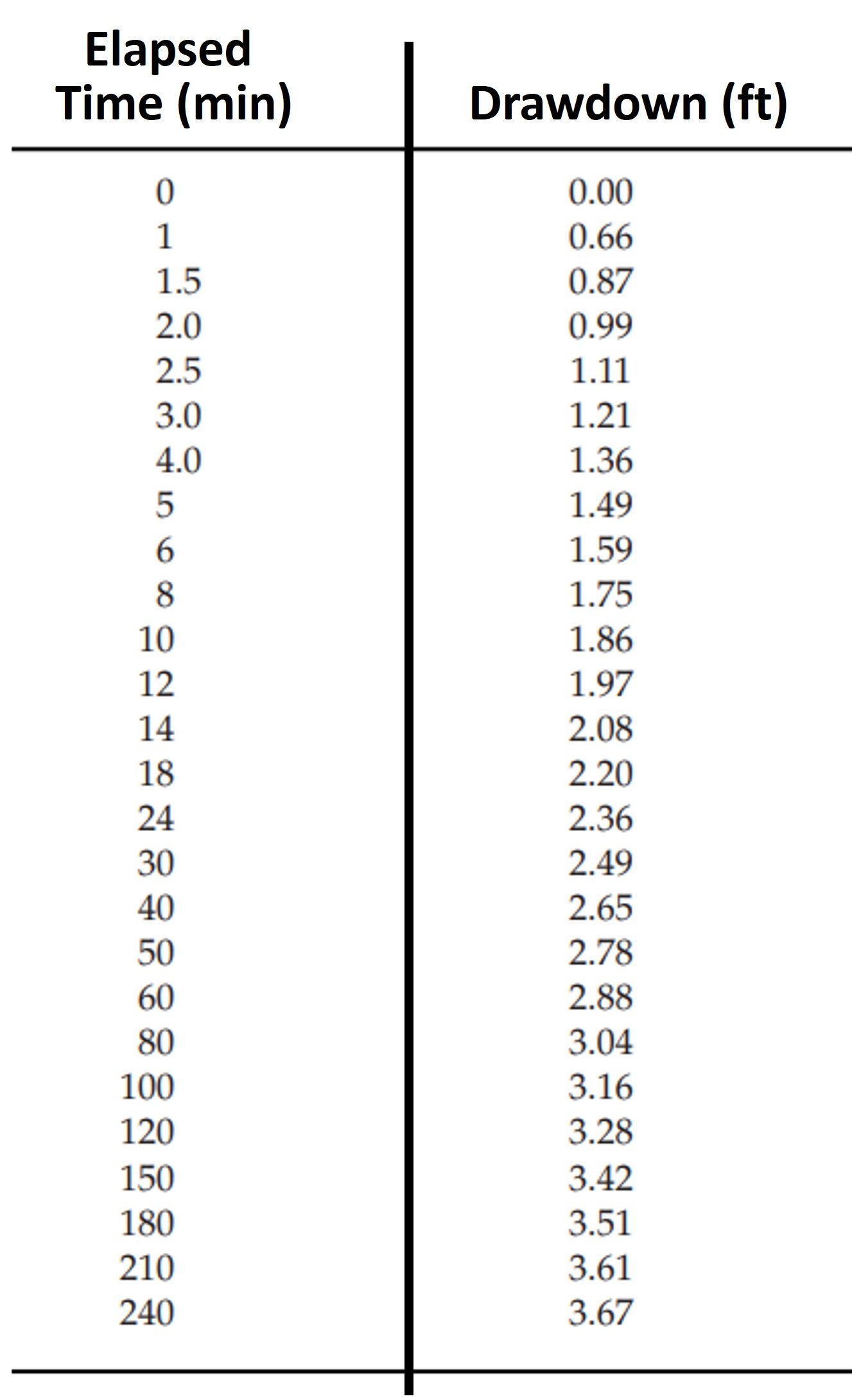
The data are plotted using MATLAB code cooperjacob.m, which can be found in the Google Drive folder mentioned in the beginning of the post.

Noting that one cycle covers a drawdown interval $\displaystyle \Delta$ s = 1.2 ft, we can use equation (14) to obtain the transmissivity T,

$\displaystyle T=\frac{{2.30Q}}{{4\pi s}}=\frac{{2.30\times 0.45}}{{4\pi \times 1.2}}=0.0686\,\,\text{f}{{\text{t}}^{2}}\text{/s}$

$\displaystyle \therefore T=5930\,\,\text{f}{{\text{t}}^{2}}\text{/day}\leftarrow$

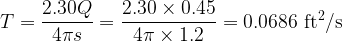
Now, the horizontal intercept of the drawdown data is t₀ = 0.35 min. Noting that 1 day = 1440 min and substituting into equation (16) gives, for the storativity S,

$\displaystyle S=\frac{{2.25T{{t}_{0}}}}{{{{r}^{2}}}}=\frac{{2.25\times 5930\times \left( {{{0.35}}/{{1440}}\;} \right)}}{{{{{240}}^{2}}}}=5.63\times {{10}^{{-5}}}\leftarrow$

3. The Hantush-Jacob solution for wells in a leaky, semiconfined aquifer

Most aquifers are not isolated from sources of vertical recharge. Aquitards, either above or below the aquifer, can leak water into the aquifer if the direction of the hydraulic gradient is favorable. An aquifer overlain by a permeable confining layer is known as a leaky aquifer. Unsteady drawdown due to a constant-rate pumping well in this type of aquifer can be assessed with the Hantush-Jacob model. The governing equation those authors worked with was (see Figure 3)

$\displaystyle \frac{S}{T}\frac{{\partial s}}{{\partial t}}=\frac{1}{r}\frac{d}{{dr}}\left( {r\frac{{ds}}{{dr}}} \right)-\frac{s}{{{{\lambda }^{2}}}}\,\,\,(20)$

Here, $\displaystyle \lambda$ is a parameter known as the leakage factor,

$\displaystyle \lambda =\sqrt{{\frac{{{b}'T}}{{{K}'}}}}\,\,\,(21)$

where b’ is the thickness of the aquitard, T is the transmissivity of the confined aquifer, and K’ is the hydraulic conductivity of the aquitard. Clearly, the leakage factor is a combined property of the aquifer and aquitard. As noted by Cheng (2000), the ratio b’/K’ is an aquitard property called the leakage coefficient or leakance. Its inverse, b’/K’, is known as the hydraulic resistance. The leakage coefficient represents the aquitard flow across a unit horizontal area into the adjacent aquifer under a unit head difference between the top and bottom of the aquitard.

Hantush and Jacob assumed that all the water flowing to the pumping well came from either elastic storage in the confined aquifer or leakage across the confining layer. No water is derived from elastic storage in the confining layer. To summarize, the assumptions used by those authors include:

The aquifer is bounded on the top by an aquitard.
The aquitard is overlain by an unconfined aquifer, known as the source bed.
The water table in the source bed is initially horizontal.
The water table in the source bed does not fall during pumping of the aquifer.
Groundwater flow in the aquitard is vertical.
The aquifer is compressible, and water drains instantaneously with a decline in head.
The aquitard is incompressible, so that no water is released from storage in the aquitard when the aquifer is pumped.

The solution to (20) obtained by Hantush and Jacob is

$\displaystyle s=\frac{Q}{{4\pi T}}{{W}_{{HJ}}}\left( {u,\frac{r}{\lambda }} \right)\,\,\,(22)$

Here, W_HJ is the Hantush-Jacob leaky aquifer well function, which is expressed as

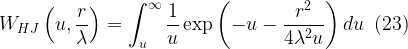
$\displaystyle {{W}_{{HJ}}}\left( {u,\frac{r}{\lambda }} \right)=\int_{u}^{\infty }{{\frac{1}{u}\exp \left( {-u-\frac{{{{r}^{2}}}}{{4{{\lambda }^{2}}u}}} \right)du}}\,\,\,(23)$

where u is the same parameter used in the Theis solution.

Figure 3. Well in a leaky aquifer.

Example problem 3

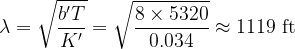
If the aquifer described in example problem 1 is not fully confined, but is overlain by a 8.0-ft thick leaky, confining layer with a vertical hydraulic conductivity of 0.034 ft/day, what would be the drawdown values after 30 days of pumping at 165,000 ft³/day at the indicated distances?

As an example, we shall carry out the calculations for r = 500 ft. We first compute argument u (whose value is identical to the one obtained in problem 1),

$\displaystyle u=\frac{{{{r}^{2}}S}}{{4Tt}}=\frac{{{{{500}}^{2}}\times 0.0007}}{{4\times 5320\times 30}}=2.74\times {{10}^{{-4}}}$

Next, we compute the leakage factor $\displaystyle \lambda$ ,

$\displaystyle \lambda =\sqrt{{\frac{{{b}'T}}{{{K}'}}}}=\sqrt{{\frac{{8\times 5320}}{{0.034}}}}\approx 1119\,\,\text{ft}$

Then, we proceed to compute the leaky aquifer well function W_HJ(u,r/ $\displaystyle \lambda$ ). There is no analytical solution to the integral that defines W_HJ(u, r/ $\displaystyle \lambda$ ), but we can easily approximate the integral numerically; in code hantushjacob.m, we use MATLAB’s Symbolic Math Toolbox to declare the integral symbolically and then apply the function vpa() to evaluate the integral numerically. For the example at hand,

$\displaystyle {{W}_{{HJ}}}\left( {u=2.74\times {{{10}}^{{-4}}},\frac{r}{\lambda }=\frac{{500}}{{1119}}} \right)=2.038$

Lastly, the drawdown s is determined as

$\displaystyle s=\frac{Q}{{4\pi T}}{{W}_{{HJ}}}\left( u \right)=\frac{{165,000}}{{4\pi \times 5320}}\times 2.038=5.03\,\,\text{ft}$

Thus, after 30 days of pumping the drawdown at a distance of 500 ft from the well equals 5.03 ft. Similar calculations apply to other values of radial distance. The calculations are automated in hantushjacob.m. The drawdown-versus-distance plot is shown below.

References

CHENG, A.H.-D. (2000). Multilayered Aquifer Systems. Marcel Dekker.
FETTER, C.W., Jr. (2014). Applied Hydrogeology. 4th edition. Pearson.
GUPTA, R.S. (2017). Hydrology and Hydraulic Systems. 4th edition. Waveland Press.

Drawdown in Aquifers: Theis and Hantush-Jacob Well Functions

Subscribe to our Mailing List!

Featured Posts

A Primer on NAND Flash Memories

Solidification Time and Chvorinov’s Rule

Step-Growth Polymerization, the Carothers Equation, and the Flory-Schulz Distribution

More Articles

Four Models for One-Dimensional Infiltration of Water in Soils

Harmful Algal Blooms and Lake Restoration

Fields of Study

More

© 2024 Montogue Quiz

Subscribe to
our Mailing List!

Subscribe to our Mailing List!

Subscribe to receive our latest materials in your inbox.

Homework Help

© 2024 Montogue Quiz

Subscribe to our Mailing List!