
All introductory optics courses cover diffraction phenomena, and most begin their coverage of this topic with Fraunhofer diffraction. In Fraunhofer diffraction, the source and screen are arranged to be effectively at infinity from the diffraction device, a slit-like aperture, or a diffraction grating. This simplifies the treatment appreciably because the emitted waves reach the apertures as plane waves, all having the same phase and amplitude. We do away with these limitations in near-field, or Fresnel, diffraction, so named after the French engineer and physicist Augustin-Jean Fresnel (1788 – 1827). In this post, I provide a quick introduction to this phenomenon, with emphasis on the concepts of Fresnel zones and Fresnel integrals. Two solved examples are included along the way.
1. Obliquity factor
A crucial aspect of Fresnel diffraction is that waves emitted by a point source at a finite distance from an aperture or a straight-edge obstacle are spherical in nature. As light diffracts through the opening, points on the primary wavefront are envisioned as continuous emitters of secondary spherical wavelets; this is illustrated in Figure 1.
Figure 1. Near-field diffraction along an aperture.
But if each wavelet radiated uniformly in all directions, in addition to generating an ongoing wave, there would also be a reverse wave travelling back toward the source. Since no such wave is found experimentally, we must somehow modify the radiation pattern of the secondary emitters. With this goal in mind, we introduce a quantity called the obliquity factor F(

In this equation,
2. Basics of Fresnel diffraction
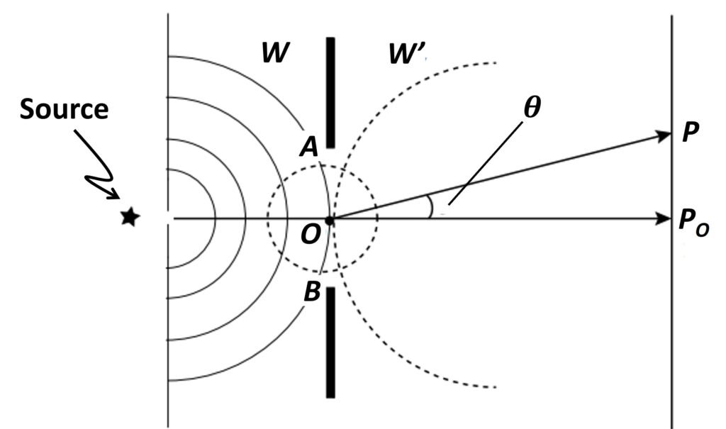
To develop a mathematical treatment of Fresnel diffraction, we refer to Figure 2, where arc WW represents a primary wave with a spherical wave front of radius 


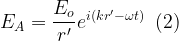
where t is time and 

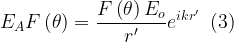
The wave in equation (3) propagates to a receiving point P as a secondary wavelet of an element of disturbance dEp given by

Combining equations (3) and (4) gives the disturbance at a point P due to the wavelets reaching P, that is,
![\displaystyle d{{E}_{P}}=\frac{{F\left( \theta \right){{E}_{o}}}}{{r{r}'}}{{e}^{{i\left[ {k\left( {r+{r}'} \right)-\omega t} \right]}}}\,\,\,(5)](https://s0.wp.com/latex.php?latex=%5Cdisplaystyle+d%7B%7BE%7D_%7BP%7D%7D%3D%5Cfrac%7B%7BF%5Cleft%28+%5Ctheta+%5Cright%29%7B%7BE%7D_%7Bo%7D%7D%7D%7D%7B%7Br%7Br%7D%27%7D%7D%7B%7Be%7D%5E%7B%7Bi%5Cleft%5B+%7Bk%5Cleft%28+%7Br%2B%7Br%7D%27%7D+%5Cright%29-%5Comega+t%7D+%5Cright%5D%7D%7D%7D%5C%2C%5C%2C%5C%2C%285%29&bg=ffffff&fg=000&s=1&c=20201002)
To include contributions of all wavelets generated by the aperture points, we integrate over the area A:
![\displaystyle {{E}_{P}}=\int_{A}{{\frac{{F\left( \theta \right){{E}_{o}}}}{{r{r}'}}{{e}^{{i\left[ {k\left( {r+{r}'} \right)-\omega t} \right]}}}dA}}\,\,\,(6)](https://s0.wp.com/latex.php?latex=%5Cdisplaystyle+%7B%7BE%7D_%7BP%7D%7D%3D%5Cint_%7BA%7D%7B%7B%5Cfrac%7B%7BF%5Cleft%28+%5Ctheta+%5Cright%29%7B%7BE%7D_%7Bo%7D%7D%7D%7D%7B%7Br%7Br%7D%27%7D%7D%7B%7Be%7D%5E%7B%7Bi%5Cleft%5B+%7Bk%5Cleft%28+%7Br%2B%7Br%7D%27%7D+%5Cright%29-%5Comega+t%7D+%5Cright%5D%7D%7D%7DdA%7D%7D%5C%2C%5C%2C%5C%2C%286%29&bg=ffffff&fg=000&s=1&c=20201002)
Figure 2. Spherical wavefront emitted by a source, S.
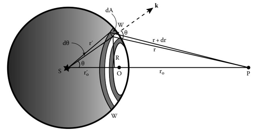
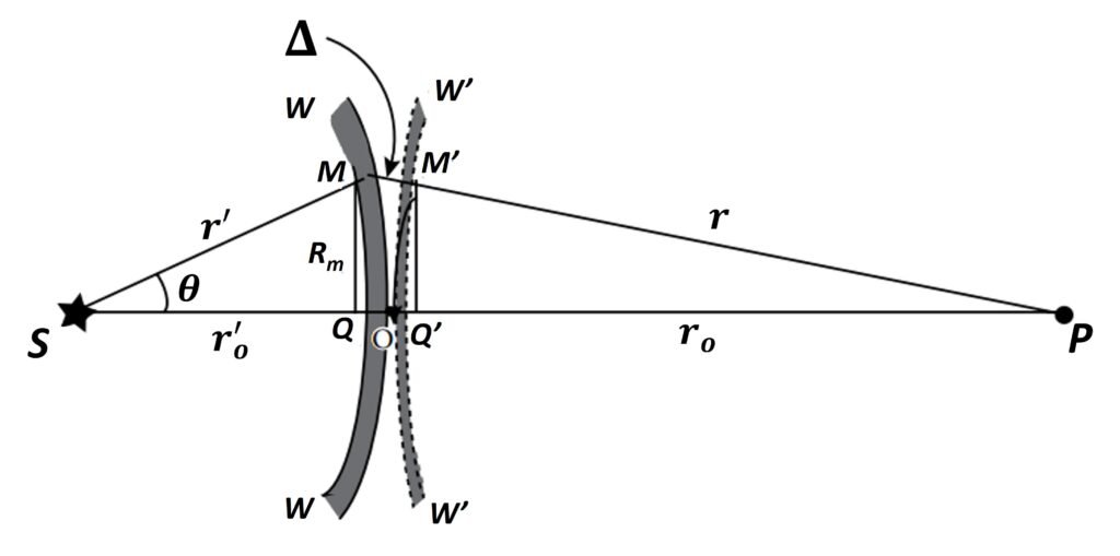
Figure 3. Path difference along SP and SMM’P.
In an attempt to carry out the integration in (6), Fresnel introduced a special construction of the primary incident wave that encounters the apertures as it propagates. In his scheme, the incident wavefront is divided into zones of circles that have a finite width centered on the pole O. The circles are constructed such that the distance from the observation point P to the first (smallest) circle is r + 
For a simple implementation of such a process, refer to Figure 3, in which we have a side view of an aperture, a segment of a Fresnel zone on a primary wave, and a wavelet generated at a point of the aperture. Consider the two points O and M through which the paths SOP and SMP pass. The first is the shortest path of light between the source and receiving point P traversed by the primary wave and the secondary wavelet generated at O. The second is the path OM plus that of a wavelet generated at M, another point on the primary wave. The two paths, being not equal, are of a path difference 

which can be stated as

Segments QO and Q’O are known as the sagittas of the arcs WW and W’W’. For a small height of points M and M’ above the line SOP, these heights can be shown to equal
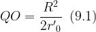

so that (8) becomes

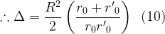
But the path difference

Equating (10) and (11) and solving for Rm, (i.e., the value of R at the m-th order), we have

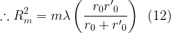
But, from the geometry of Figure 3, we also have

so that, equating (12) and (13) and manipulating,
![\displaystyle R_{m}^{2}=r_{0}^{2}\left[ {\left( {\frac{{m\lambda }}{{{{r}_{0}}}}} \right)+{{{\left( {\frac{{m\lambda }}{{2{{r}_{0}}}}} \right)}}^{2}}} \right]\,\,\,(14)](https://s0.wp.com/latex.php?latex=%5Cdisplaystyle+R_%7Bm%7D%5E%7B2%7D%3Dr_%7B0%7D%5E%7B2%7D%5Cleft%5B+%7B%5Cleft%28+%7B%5Cfrac%7B%7Bm%5Clambda+%7D%7D%7B%7B%7B%7Br%7D_%7B0%7D%7D%7D%7D%7D+%5Cright%29%2B%7B%7B%7B%5Cleft%28+%7B%5Cfrac%7B%7Bm%5Clambda+%7D%7D%7B%7B2%7B%7Br%7D_%7B0%7D%7D%7D%7D%7D+%5Cright%29%7D%7D%5E%7B2%7D%7D%7D+%5Cright%5D%5C%2C%5C%2C%5C%2C%2814%29&bg=ffffff&fg=000&s=1&c=20201002)
But m
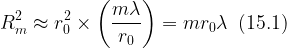
or

This equation indicates that the radius of a given Fresnel zone is proportional to the square root of its order m. For an aperture of radius a, whose center is on the line connecting the source and the observation point P, the number of zones N that pass through the aperture can be calculated as

where Am is the area of the m-th zone. Letting the central zone (the first zone) be labelled m = 1, we have A1 = 


Number N may be used to distinguish Fraunhofer diffraction from Fresnel diffraction: if N
Example 1
Consider a monochromatic light of wavelength
(a) The radius of the central zone.
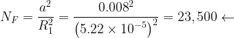
(b) The number of Fresnel zones that would be accommodated through the aperture.
Solution, Part a. We have m = 1, 


Part b. The number N of Fresnel zones that would pass through the aperture is given by equation (17),
4. Fresnel diffraction in a rectangular aperture – Analytical treatment
We now turn to an analytical treatment of Fresnel diffraction for a rectangular aperture. As shown in Figure 4, we begin by taking an elemental strip chosen along the width W of the rectangular aperture. A spherical wave incident on a very large number of these strips would constitute a problem in requiring the phase at all points of the strip to be constant; harder still would be to require the phase to be the same along successive elemental strips. One way to remedy this is to have a cylindrical source parallel to the aperture plane, so that all points of the cylindrical wave front would have the same phase. Aside from the geometry of the aperture, which requires the source to be an extended slit so that cylindrical waves are considered, no constraints are applied and the Fresnel equation (6) can be restated as

where all constants are gleaned into a parameter C1. We assume that the surface integral over a closed surface including the aperture is zero everywhere except over the aperture itself, so that we need perform the integration only over the aperture in the yz-plane of Figure 4a. A side view, which shows the curvature of the cylindrical wavefront, is drawn in Figure 4b.
Figure 4. (a) Cylindrical wavefronts from source slit S are diffracted by a rectangular aperture. (b) Edge view of (a).
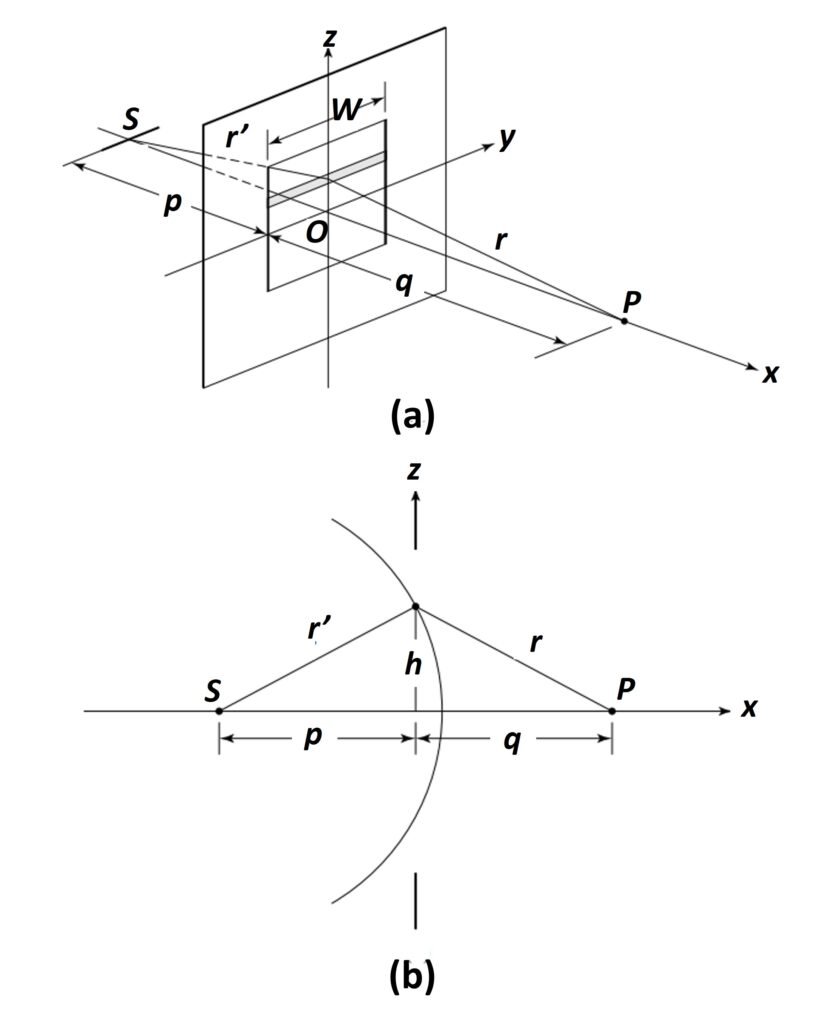
The distance r + r’ may be determined approximately from this figure. For h

so that

Proceeding similarly with r,

Adding the two foregoing results,

For convenience, we introduce the variables

and

so that

If the elemental area dA is taken to be the shaded strip in Figure 4, dA = Wdz, h = z, and
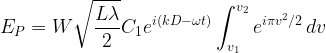
The exponent in the integrand can be restated as

where k is wavenumber and

or

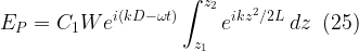
so we can restate (25) as

where Ap is a complex scale factor with dimensions of electric field amplitude. Using Euler’s theorem on the integrand, it follows that
![\displaystyle {{E}_{P}}={{A}_{P}}{{e}^{{i\left( {kD-\omega t} \right)}}}\left[ {\int_{{{{v}_{1}}}}^{{{{v}_{2}}}}{{\cos \left( {\frac{{\pi {{v}^{2}}}}{2}} \right)dv}}+i\times \int_{{{{v}_{1}}}}^{{{{v}_{2}}}}{{\sin \left( {\frac{{\pi {{v}^{2}}}}{2}} \right)dv}}} \right]\,\,\,(29)](https://s0.wp.com/latex.php?latex=%5Cdisplaystyle+%7B%7BE%7D_%7BP%7D%7D%3D%7B%7BA%7D_%7BP%7D%7D%7B%7Be%7D%5E%7B%7Bi%5Cleft%28+%7BkD-%5Comega+t%7D+%5Cright%29%7D%7D%7D%5Cleft%5B+%7B%5Cint_%7B%7B%7B%7Bv%7D_%7B1%7D%7D%7D%7D%5E%7B%7B%7B%7Bv%7D_%7B2%7D%7D%7D%7D%7B%7B%5Ccos+%5Cleft%28+%7B%5Cfrac%7B%7B%5Cpi+%7B%7Bv%7D%5E%7B2%7D%7D%7D%7D%7B2%7D%7D+%5Cright%29dv%7D%7D%2Bi%5Ctimes+%5Cint_%7B%7B%7B%7Bv%7D_%7B1%7D%7D%7D%7D%5E%7B%7B%7B%7Bv%7D_%7B2%7D%7D%7D%7D%7B%7B%5Csin+%5Cleft%28+%7B%5Cfrac%7B%7B%5Cpi+%7B%7Bv%7D%5E%7B2%7D%7D%7D%7D%7B2%7D%7D+%5Cright%29dv%7D%7D%7D+%5Cright%5D%5C%2C%5C%2C%5C%2C%2829%29&bg=ffffff&fg=000&s=1&c=20201002)
The two integrals on the right-hand side are known as Fresnel integrals, and are routinely denoted with the simplified notations
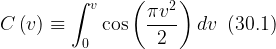
and

Substituting these into (29) gives
![\displaystyle {{E}_{P}}={{A}_{P}}{{e}^{{i\left( {kD-\omega t} \right)}}}\left\{ {\left[ {C\left( {{{v}_{2}}} \right)-C\left( {{{v}_{1}}} \right)} \right]+i\left[ {S\left( {{{v}_{2}}} \right)-S\left( {{{v}_{1}}} \right)} \right]} \right\}\,\,\,(31)](https://s0.wp.com/latex.php?latex=%5Cdisplaystyle+%7B%7BE%7D_%7BP%7D%7D%3D%7B%7BA%7D_%7BP%7D%7D%7B%7Be%7D%5E%7B%7Bi%5Cleft%28+%7BkD-%5Comega+t%7D+%5Cright%29%7D%7D%7D%5Cleft%5C%7B+%7B%5Cleft%5B+%7BC%5Cleft%28+%7B%7B%7Bv%7D_%7B2%7D%7D%7D+%5Cright%29-C%5Cleft%28+%7B%7B%7Bv%7D_%7B1%7D%7D%7D+%5Cright%29%7D+%5Cright%5D%2Bi%5Cleft%5B+%7BS%5Cleft%28+%7B%7B%7Bv%7D_%7B2%7D%7D%7D+%5Cright%29-S%5Cleft%28+%7B%7B%7Bv%7D_%7B1%7D%7D%7D+%5Cright%29%7D+%5Cright%5D%7D+%5Cright%5C%7D%5C%2C%5C%2C%5C%2C%2831%29&bg=ffffff&fg=000&s=1&c=20201002)
Now, note that the irradiance at P is given by
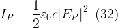
where 

![\displaystyle {{I}_{P}}={{I}_{0}}\left\{ {{{{\left[ {C\left( {{{v}_{2}}} \right)-C\left( {{{v}_{1}}} \right)} \right]}}^{2}}+{{{\left[ {S\left( {{{v}_{2}}} \right)-S\left( {{{v}_{1}}} \right)} \right]}}^{2}}} \right\}\,\,\,(33)](https://s0.wp.com/latex.php?latex=%5Cdisplaystyle+%7B%7BI%7D_%7BP%7D%7D%3D%7B%7BI%7D_%7B0%7D%7D%5Cleft%5C%7B+%7B%7B%7B%7B%5Cleft%5B+%7BC%5Cleft%28+%7B%7B%7Bv%7D_%7B2%7D%7D%7D+%5Cright%29-C%5Cleft%28+%7B%7B%7Bv%7D_%7B1%7D%7D%7D+%5Cright%29%7D+%5Cright%5D%7D%7D%5E%7B2%7D%7D%2B%7B%7B%7B%5Cleft%5B+%7BS%5Cleft%28+%7B%7B%7Bv%7D_%7B2%7D%7D%7D+%5Cright%29-S%5Cleft%28+%7B%7B%7Bv%7D_%7B1%7D%7D%7D+%5Cright%29%7D+%5Cright%5D%7D%7D%5E%7B2%7D%7D%7D+%5Cright%5C%7D%5C%2C%5C%2C%5C%2C%2833%29&bg=ffffff&fg=000&s=1&c=20201002)
where we have introduced the irradiance scale factor 

It is important to note that C(v) and S(v) are both odd functions, so that


The choice of v in the Fresnel integrals is determined by the vertical dimensions of the diffraction aperture.
Some values of the Fresnel integrals are listed here. Tabulated values are convenient, but often require tedious interpolation. A better alternative is to use software such as Mathematica or MATLAB, or resort to this free web-based app by Casio.
5. The Cornu spiral
If the values of the Fresnel integrals are plotted with C(v) on the horizontal axis and S(v) on the vertical axis, the resulting graph is the so-called Cornu spiral, Figure 5. The origin v = 0 of the Cornu spiral corresponds to z = 0 and therefore to the y-axis through the aperture of Figure 4. The top part of the spiral (z > 0 and v > 0) represents contributions from strips of the aperture above the y-axis, and the twin spiral below (z < 0 and v < 0) represents similar contributions from below the y-axis. The two limit points or “eyes” of the spiral at E and E’ represent linear zones at z = 

Furthermore, variable v, introduced in (27.2), represents the length along the Cornu spiral itself. To see this, recall that the incremental length dl along a curve in the xy-plane is given by the Pythagorean relationship

But in the Cornu spiral plane the x– and y-coordinates are given by the Fresnel integrals C(v) and S(v), respectively, giving
![\displaystyle d{{l}^{2}}={{\left[ {dC\left( v \right)} \right]}^{2}}+{{\left[ {dS\left( v \right)} \right]}^{2}}](https://s0.wp.com/latex.php?latex=%5Cdisplaystyle+d%7B%7Bl%7D%5E%7B2%7D%7D%3D%7B%7B%5Cleft%5B+%7BdC%5Cleft%28+v+%5Cright%29%7D+%5Cright%5D%7D%5E%7B2%7D%7D%2B%7B%7B%5Cleft%5B+%7BdS%5Cleft%28+v+%5Cright%29%7D+%5Cright%5D%7D%5E%7B2%7D%7D&bg=ffffff&fg=000&s=1&c=20201002)
![\displaystyle \therefore d{{l}^{2}}=\left[ {{{{\cos }}^{2}}\left( {\frac{{\pi {{v}^{2}}}}{2}} \right)+{{{\sin }}^{2}}\left( {\frac{{\pi {{v}^{2}}}}{2}} \right)} \right]d{{v}^{2}}](https://s0.wp.com/latex.php?latex=%5Cdisplaystyle+%5Ctherefore+d%7B%7Bl%7D%5E%7B2%7D%7D%3D%5Cleft%5B+%7B%7B%7B%7B%5Ccos+%7D%7D%5E%7B2%7D%7D%5Cleft%28+%7B%5Cfrac%7B%7B%5Cpi+%7B%7Bv%7D%5E%7B2%7D%7D%7D%7D%7B2%7D%7D+%5Cright%29%2B%7B%7B%7B%5Csin+%7D%7D%5E%7B2%7D%7D%5Cleft%28+%7B%5Cfrac%7B%7B%5Cpi+%7B%7Bv%7D%5E%7B2%7D%7D%7D%7D%7B2%7D%7D+%5Cright%29%7D+%5Cright%5Dd%7B%7Bv%7D%5E%7B2%7D%7D&bg=ffffff&fg=000&s=1&c=20201002)


Another noteworthy feature of the Cornu spiral is that its tangent at a certain point (x, y) is given by the tangent of variable 
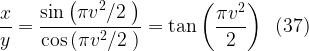
Figure 5. A Cornu spiral.

6. Unobstructed wavefront
The irradiance in the Fresnel diffraction pattern associated with different apertures are often compared to the irradiance Iu associated with an unobstructed wavefront. An unobstructed wavefront is modeled by passage through an aperture with a vertical dimension 2 that ranges from ‒∞ to +∞. In this case, the total irradiance Iu at point P is proportional to the square of the length of the phasor drawn from E’ to E in Figure 5. These limiting points have coordinates (C(v2), S(v2)) = (0.5, 0.5) and (C(v1), S(v1)) = (‒0.5, ‒0.5), as given by the improper integrals
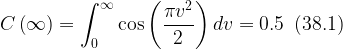

and from the fact that C(v) and S(v) are odd functions. It follows that, substituting into (33), the unobstructed irradiance becomes
![\displaystyle {{I}_{u}}={{I}_{0}}\left\{ {{{{\left[ {C\left( \infty \right)-C\left( {-\infty } \right)} \right]}}^{2}}+{{{\left[ {S\left( \infty \right)-S\left( {-\infty } \right)} \right]}}^{2}}} \right\}](https://s0.wp.com/latex.php?latex=%5Cdisplaystyle+%7B%7BI%7D_%7Bu%7D%7D%3D%7B%7BI%7D_%7B0%7D%7D%5Cleft%5C%7B+%7B%7B%7B%7B%5Cleft%5B+%7BC%5Cleft%28+%5Cinfty+%5Cright%29-C%5Cleft%28+%7B-%5Cinfty+%7D+%5Cright%29%7D+%5Cright%5D%7D%7D%5E%7B2%7D%7D%2B%7B%7B%7B%5Cleft%5B+%7BS%5Cleft%28+%5Cinfty+%5Cright%29-S%5Cleft%28+%7B-%5Cinfty+%7D+%5Cright%29%7D+%5Cright%5D%7D%7D%5E%7B2%7D%7D%7D+%5Cright%5C%7D&bg=ffffff&fg=000&s=1&c=20201002)
![\displaystyle \therefore {{I}_{u}}={{I}_{0}}\left\{ {{{{\left[ {0.5-\left( {-0.5} \right)} \right]}}^{2}}+{{{\left[ {0.5-\left( {-0.5} \right)} \right]}}^{2}}} \right\}](https://s0.wp.com/latex.php?latex=%5Cdisplaystyle+%5Ctherefore+%7B%7BI%7D_%7Bu%7D%7D%3D%7B%7BI%7D_%7B0%7D%7D%5Cleft%5C%7B+%7B%7B%7B%7B%5Cleft%5B+%7B0.5-%5Cleft%28+%7B-0.5%7D+%5Cright%29%7D+%5Cright%5D%7D%7D%5E%7B2%7D%7D%2B%7B%7B%7B%5Cleft%5B+%7B0.5-%5Cleft%28+%7B-0.5%7D+%5Cright%29%7D+%5Cright%5D%7D%7D%5E%7B2%7D%7D%7D+%5Cright%5C%7D&bg=ffffff&fg=000&s=1&c=20201002)

Other irradiances may be compared conveniently to this result.
Example 2
A slit illuminated with sodium light (
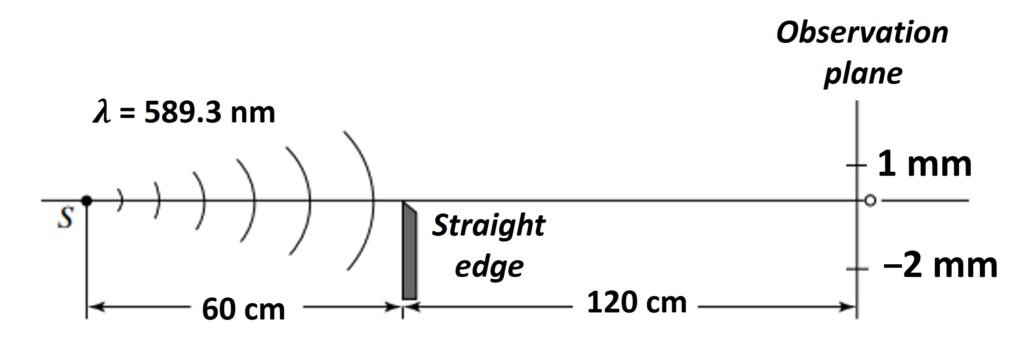
Solution, Part a. For either position, parameter L is such that (equation (23))


Let z’ be the coordinate of the point O’ in the aperture plane along the straight line from S to the observation point P (see Figure 2). In the case at hand, with y = ‒2 mm, we may write

The values of the z1 and z2 that mark the edges of the unobstructed regions in the aperture plane are to be measured relative to this point, so z2 = ∞ and z1 = +6.67


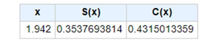
The Fresnel integrals for v2 are obvious: C(v2) = S(v2) = 0.5. In turn, entering v1 into the Casio app gives C(v1) = 0.4315 and S(v1) = 0.3538, as shown.
Referring to eq. (29), we compute the relative irradiance I:
![\displaystyle I={{I}_{0}}\left\{ {{{{\left[ {C\left( {{{v}_{2}}} \right)-C\left( {{{v}_{1}}} \right)} \right]}}^{2}}+{{{\left[ {S\left( {{{v}_{2}}} \right)-S\left( {{{v}_{1}}} \right)} \right]}}^{2}}} \right\}](https://s0.wp.com/latex.php?latex=%5Cdisplaystyle+I%3D%7B%7BI%7D_%7B0%7D%7D%5Cleft%5C%7B+%7B%7B%7B%7B%5Cleft%5B+%7BC%5Cleft%28+%7B%7B%7Bv%7D_%7B2%7D%7D%7D+%5Cright%29-C%5Cleft%28+%7B%7B%7Bv%7D_%7B1%7D%7D%7D+%5Cright%29%7D+%5Cright%5D%7D%7D%5E%7B2%7D%7D%2B%7B%7B%7B%5Cleft%5B+%7BS%5Cleft%28+%7B%7B%7Bv%7D_%7B2%7D%7D%7D+%5Cright%29-S%5Cleft%28+%7B%7B%7Bv%7D_%7B1%7D%7D%7D+%5Cright%29%7D+%5Cright%5D%7D%7D%5E%7B2%7D%7D%7D+%5Cright%5C%7D&bg=ffffff&fg=000&s=1&c=20201002)
![\displaystyle \therefore I={{I}_{0}}\left[ {{{{\left( {0.5-0.4315} \right)}}^{2}}+{{{\left( {0.5-0.3538} \right)}}^{2}}} \right]=0.0261{{I}_{0}}](https://s0.wp.com/latex.php?latex=%5Cdisplaystyle+%5Ctherefore+I%3D%7B%7BI%7D_%7B0%7D%7D%5Cleft%5B+%7B%7B%7B%7B%5Cleft%28+%7B0.5-0.4315%7D+%5Cright%29%7D%7D%5E%7B2%7D%7D%2B%7B%7B%7B%5Cleft%28+%7B0.5-0.3538%7D+%5Cright%29%7D%7D%5E%7B2%7D%7D%7D+%5Cright%5D%3D0.0261%7B%7BI%7D_%7B0%7D%7D&bg=ffffff&fg=000&s=1&c=20201002)
Comparing this with the unobstructed irradiance as given by (39), we get

Solution, Part b. In this case, z’ becomes

so that z2 = ∞ and z1 = ‒3.33
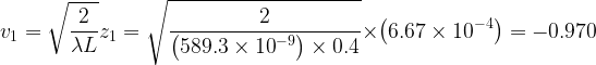
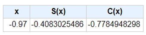
As before, the Fresnel integrals for v2 are C(v2) = S(v2) = 0.5. Next, entering v1 into the Casio calculator gives C(v1) = ‒0.7785 and S(v1) = ‒0.4083, as shown.
The relative irradiance 
![\displaystyle I={{I}_{0}}\left\{ {{{{\left[ {0.5-\left( {-0.7785} \right)} \right]}}^{2}}+{{{\left[ {0.5-\left( {-0.4083} \right)} \right]}}^{2}}} \right\}](https://s0.wp.com/latex.php?latex=%5Cdisplaystyle+I%3D%7B%7BI%7D_%7B0%7D%7D%5Cleft%5C%7B+%7B%7B%7B%7B%5Cleft%5B+%7B0.5-%5Cleft%28+%7B-0.7785%7D+%5Cright%29%7D+%5Cright%5D%7D%7D%5E%7B2%7D%7D%2B%7B%7B%7B%5Cleft%5B+%7B0.5-%5Cleft%28+%7B-0.4083%7D+%5Cright%29%7D+%5Cright%5D%7D%7D%5E%7B2%7D%7D%7D+%5Cright%5C%7D&bg=ffffff&fg=000&s=1&c=20201002)


References
- HAIJA, A.I., NUMAN, M.Z. and FREEMAN, W.L. (2018). Concise Optics: Concepts, Examples, and Problems. Boca Raton: CRC Press.
- HECHT, E. (2017). Optics. 5th edition. Upper Saddle River: Pearson.
- PEDROTTI, F.L., PEDROTTI, L.M. and PEDROTTI, L.S. (2006). Introduction to Optics. 3rd edition. Boston: Addison-Wesley.