Bagnold’s Blown Sand Transport and Saltation

1. Velocity profiles and Bagnold’s thresholds

Recall that the velocity profile in an external flow as we move away from a surface is given by the following logarithmic law, independently proposed by Prandtl and von Kármán in the first half of the 20th century.

$\displaystyle \frac{{\bar{U}}}{{u*}}=\frac{1}{\kappa }\ln \left( {\frac{z}{{{{z}_{0}}}}} \right)$

Here, $\displaystyle \bar{U}$ is flow velocity at a height z; $\displaystyle \kappa$ is the von Kármán constant, an empirical quantity often taken as 0.4 even though experimental results suggest a range of 0.33 to 0.41; $\displaystyle {{u}_{*}}$ is the so-called shear or friction velocity, which is defined as

$\displaystyle {{u}_{*}}={{\left( {\frac{{{{\tau }_{0}}}}{\rho }} \right)}^{{{1}/{2}\;}}}$

where $\displaystyle {{\tau }_{0}}$ is the shear stress at the surface and $\displaystyle \rho$ is the density of the fluid. Although $\displaystyle {{\tau }_{0}}$ has units of velocity, it is better understood as a measure of shear. In fact, it has little physical significance other than being a time-saver to avoid writing the ratio of shear to fluid density all the time.

Lastly, $\displaystyle {{z}_{0}}$ is the aerodynamic roughness length, which for sand surfaces has a typical value of 1/30 of the mean particle diameter.

When the wind velocity over a loose sand surface is slowly increased, a critical point is reached where some grains begin to move. This critical wind velocity was named the fluid threshold velocity by British explorer Ralph Bagnold. Fluid threshold velocity is defined as the lowest friction speed at which the majority of exposed particles on the surface are set in motion. According to Bagnold (1941), sand grains begin to move at a fluid threshold velocity given by

$\displaystyle {{u}_{t}}=A\sqrt{{\frac{{\left( {{{\rho }_{p}}-\rho } \right)}}{\rho }gd}}$

where $\displaystyle {{\rho }_{p}}$ is the density of the sand grain, $\displaystyle \rho$ is the density of the surrounding air, g = 9.81 m/s², d is the diameter of the sand grain, and A = 0.1 is a constant. For a 0.75-mm diameter (i.e., coarse) sand grain made of quartz in an environment at 30^oC, $\displaystyle {{\rho }_{p}}$ = 2650 kg/m³, $\displaystyle \rho$ = 1.15 kg/m³ and

$\displaystyle {{u}_{t}}=0.1\times \sqrt{{\frac{{2650-1.15}}{{1.15}}\times 9.81\times \left( {0.75\times {{{10}}^{{-3}}}} \right)}}=0.412\,\text{m/s}$

or approximately 41 cm/sec.

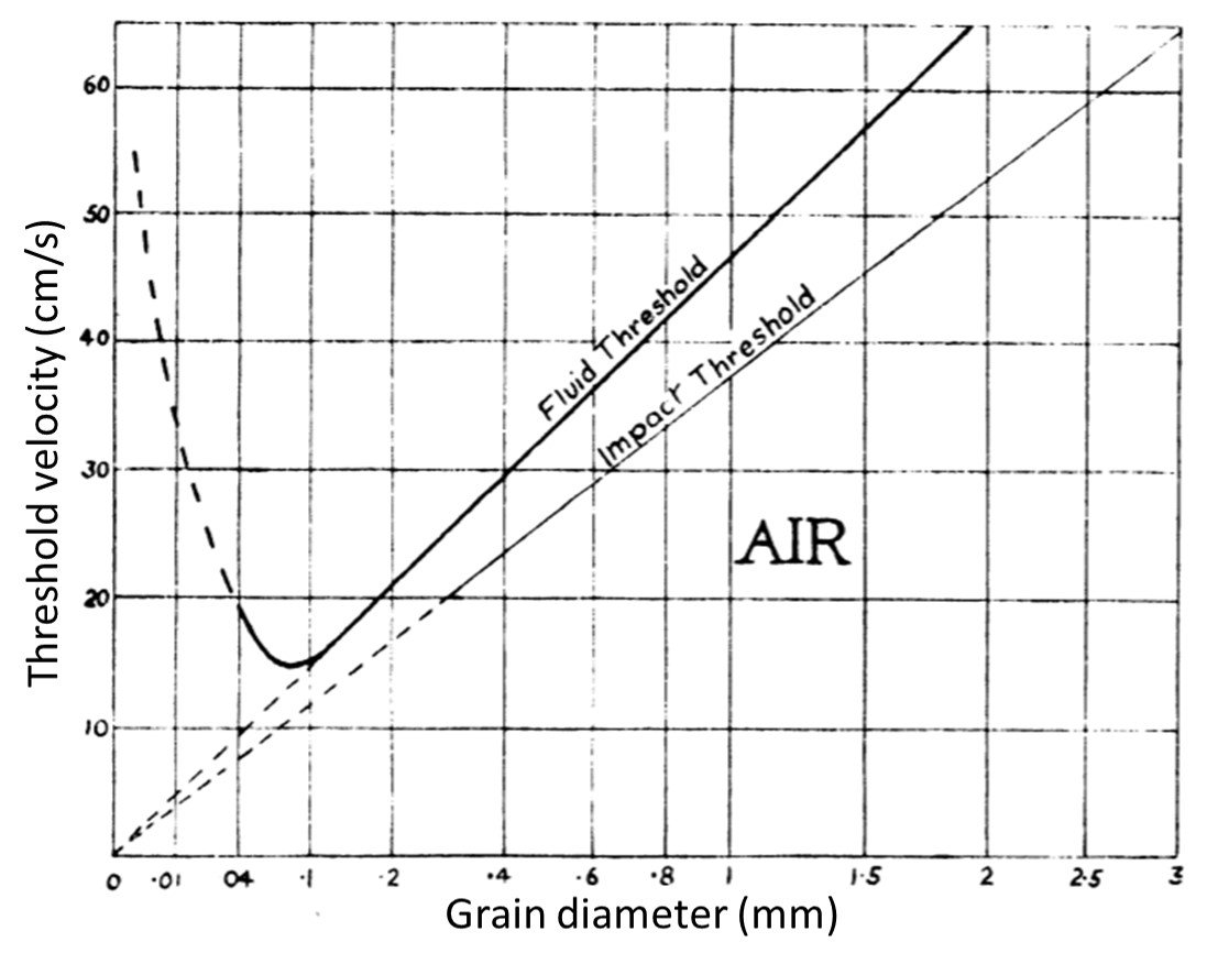
During the downwind saltation of grains, their velocity and momentum increase before they fall back to the surface. On striking the surface, the moving particles may bounce off other grains and become re-entrained into the airstream or embedded in the surface. In both cases, momentum is transferred to the surface in the disturbance of one or more stationary grains. As a result of the impact of saltating grains, particles are ejected into the airstream at shear velocities lower than that required to move a stationary grain by direct fluid pressure. This new lower threshold required to move stationary grains after the initial movement of a few particles is the impact or dynamic threshold. The impact threshold velocity for a given sediment follows the same relationship as the fluid threshold, but with a lower coefficient A = 0.08. This is illustrated in Figure 1. Notice how the impact threshold velocity is consistently lower than the fluid threshold velocity.

Figure 1. Fluid and impact threshold velocities as functions of grain size (Bagnold, 1941).

At around the same time in which von Kármán published his results on velocity profile analysis, Shields, working with aquatic sediment transport, introduced a dimensionless coefficient given by the ratio of applied tangential force to the force resisting grain movement; the so-called critical Shields parameter is given by

$\displaystyle {{\Theta }_{{\text{cr}}}}=\frac{{{{\tau }_{{0,c}}}}}{{{\rho }'gd}}$

where $\displaystyle {{\tau }_{{0,c}}}$ is the critical bed shear – the superficial shear stress at incipient grain motion – $\displaystyle {\rho }'$ is the density gradient ( $\displaystyle {{\rho }_{p}}$ – $\displaystyle \rho$ ), and d is particle size. The Bagnold parameter A is the square root of the Shields parameter at impending motion, i.e., it is the square root of the critical Shields parameter. Using empirical results obtained from flume studies, Shields plotted his parameter as a function of the particle Reynolds number, $\displaystyle {{u}_{*}}$ d/ $\displaystyle \nu$ , where $\displaystyle \nu$ is kinematic viscosity. Although the data collected by subsequent researchers showed considerable scatter, Shields’ results are usually reproduced as a single line for quantitative convenience, as shown in Figure 2. Further work carried out in wind tunnels, notably by references quoted in Sarre (1988), has generated a similar curve for Aeolian environments.

Figure 2. Plots of Shields parameter $\displaystyle \Theta$ = $\displaystyle {{A}^{2}}$ versus particle Reynolds number for liquids and air. See Sarre (1988) for references listed in the graph.

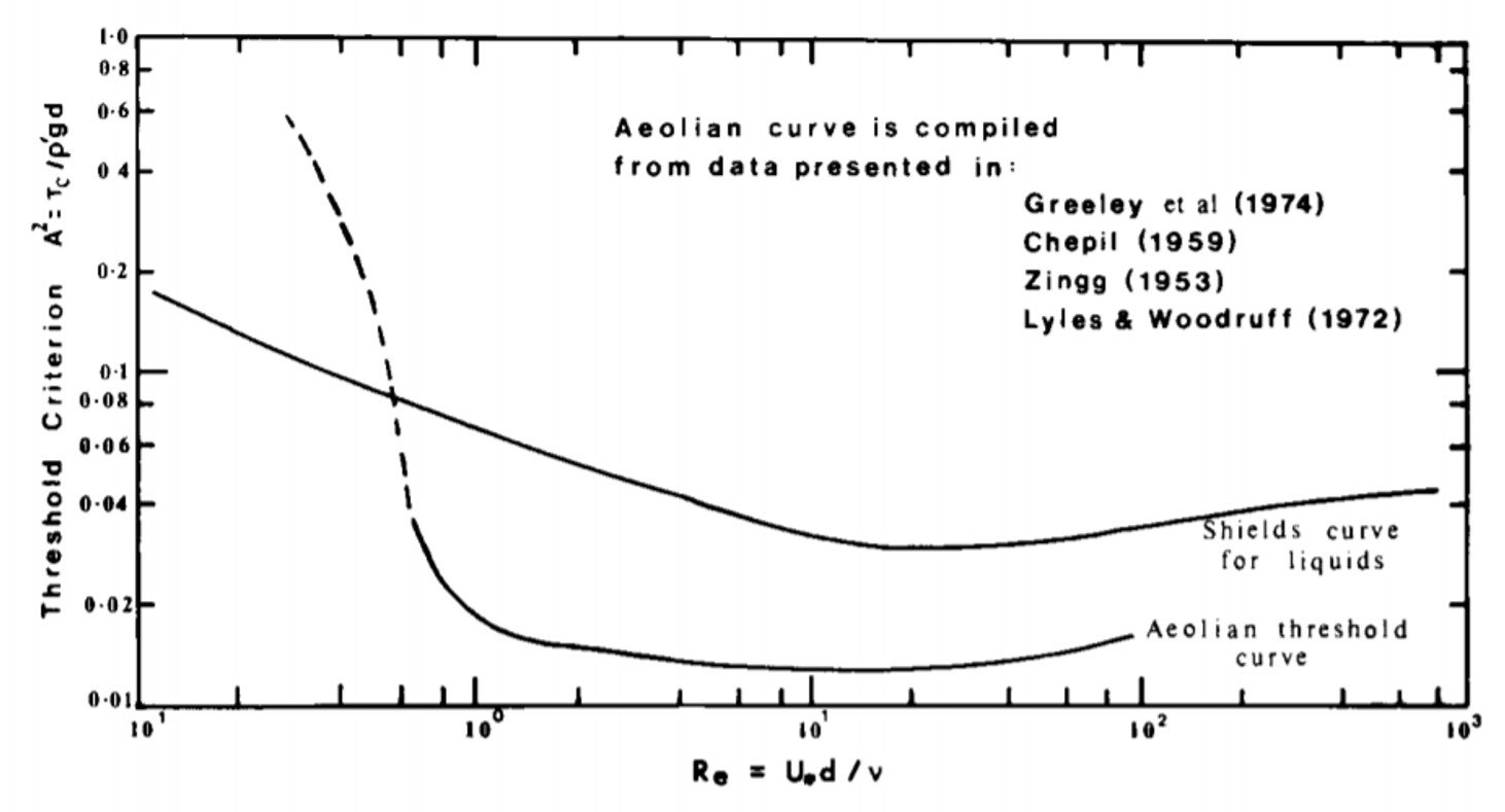
As can be seen, for values of Re greater than about 5, Bagnold’s coefficient A in air is nearly constant with a value of 0.118. For values of Re less than 5, A increases rapidly with decreasing Re. This behavior is probably due to the presence at low friction Reynolds numbers of a viscous sublayer which, in effect, shields the surface from turbulent fluctuations present in the flow. For particles of small diameter it is likely that cohesive forces, possibly due to adsorbed water films, also contribute to the higher A values. Studies published in the 1970s (e.g., Iversen et al. (1976)) confirmed the suggestion that the sharp upturn in threshold speed for small particles is attributable to particle cohesion.

2. Why saltation and not suspension? (Herrmann, 2004)

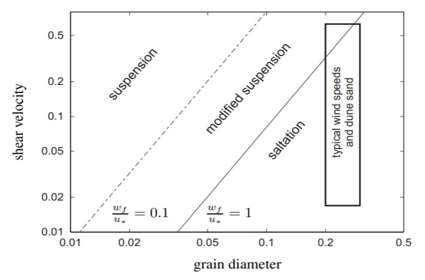
Sand grains are suspended in air if they travel long distances on irregular trajectories before reaching the ground again. A turbulent air flow can keep grains in suspension if the vertical component of the turbulent fluctuations, W’, exceeds the settling velocity W_f of the grains. Such is the case in some sandstorms, especially when shear velocities are high (say, 0.18 – 0.6 m/s) and particle diameters are relatively small (say, in the range of 0.04 – 0.06 mm). However, for wind velocities (0.2 m/s < $\displaystyle {{u}_{*}}$ < 0.6 m/s) and dune sand sizes (0.2 mm < d < 0.3 mm) that prevail in most Earthly arid environments, saltation outstrips suspension as the main bed-load transport mechanism. Figure 3 outlines the main bed-load transport types as functions of shear velocity and grain size; as shown by the vertical rectangle, conditions associated with most of the planet’s sandy environments are mainly encompassed by the saltation area of the plot. This is one of the reasons why we emphasize bed-load transport by saltation, to the detriment of suspension, in the upcoming paragraphs.

Figure 3. Mechanisms of sand transport as a function of shear velocity and grain size. The vertical rectangle indicates ranges typical of Earth’s arid environments.

Sediment transport by saltation is initiated when some grains are directly entrained by the air, a process called direct aerodynamic entrainment. If there is already a sufficiently high number of grains in the air, direct aerodynamic entrainment is negligible and grains are mainly ejected by collisions of impacting grains. After a period of transient adjustment to the overlying wind field, saltation tends to reach a constant transport rate (Owen, 1964). Most analyses of saltation consider spherical particles and two-dimensional trajectories. Once the particle initiates saltation, its trajectory can be approximated by a simple parabolic equation that should be familiar to students with some background on classical mechanics. The flight time and maximum height associated with the trajectory are then

$\displaystyle T=\frac{{2{{W}_{0}}}}{g}\,\,\,;\,\,\,h=\frac{{{{W}_{0}}}}{{2g}}$

where W₀ is the vertical component of the initial velocity. More elaborate analytical calculations such as those of Sørensen (1991) have shown that the simple approximations above can yield values up to 20% too high or too low. Wind tunnel experiments performed by Nalpanis et al. (1993) led to the useful empirical approximations

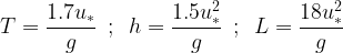
$\displaystyle T=\frac{{1.7{{u}_{*}}}}{g}\,\,\,;\,\,\,h=\frac{{1.5u_{*}^{2}}}{g}\,\,\,;\,\,\,L=\frac{{18u_{*}^{2}}}{g}$

where, in addition to T and h, we have the saltation length L. For a shear velocity of 0.4 m/s, we’d have a flight time T = 0.07 s, a hop height h = 2.45 cm, and a hop length L = 29.4 cm.

3. Adapting velocity profiles to Aeolian saltation: Bagnold’s kink (Pye and Tsoar, 2009; McEwan, 1993)

As sand grains accelerate from rest they extract momentum from the wind, thereby changing the velocity profile near the ground. Wind velocity profile measurements by Bagnold over a wet surface of uniform sand, repeated when the sand dried out and became mobile, are shown in Figure 4. Whereas the wind velocity gradients over the stable sand surface converge at a point (z₀) just above the ground surface, those measured during active sand movement converge at a higher focal point, z’, 0.2 – 0.4 cm above the surface. This effect of moving sand on the near-bed wind velocity profile has been confirmed by many workers; see the references quoted in Pye and Tsoar (2009).

Figure 4. Wind velocity profiles measured by Bagnold over a bed of 0.25 mm uniform sand with (solid lines) and without (dashed lines) sand movement.

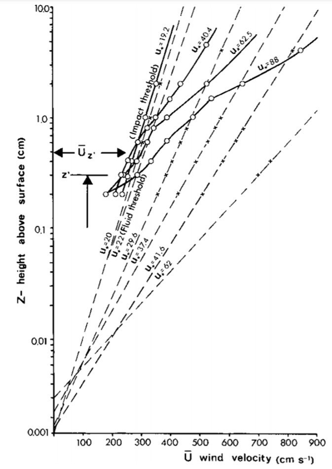
The wind profiles measured by Bagnold showed marked kinks up to a height of 3 cm, which reflect deviations from the logarithmic profile law. The width and height of the kink increase with friction velocity. Bagnold believed that these kinks correspond to the mean saltation height of uniformly sized grains. For sands with non-uniform grain size, the kink in the velocity curves is not clearly seen since different sizes have different characteristic trajectories. Some parts of the observed wind velocity profiles show negative deviations from the logarithmic velocity profile while others show positive deviations. Bagnold’s data show a negative kink (i.e., lower-than-expected velocities) at a height of 1 cm and a positive deviation (i.e., higher velocities) at a height of less than 0.5 cm. Bagnold hypothesized that the negative deviations correspond approximately to the saltation trajectory height, whereas the positive deviations reflect speeding up of the wind by the accelerating grains just before they hit the bed.

By disregarding the kinks and fitting straight lines to the velocity profile data through the focal point, Bagnold was able to rewrite the logarithmic wind velocity equation for flow over stable surfaces in a form applicable to sand surfaces on which saltation is taking place:

$\displaystyle \frac{{\bar{U}}}{{{{u}_{*}}}}=\frac{1}{\kappa }\ln \left( {\frac{z}{{{z}'}}} \right)+{{\bar{u}}_{{{z}'}}}$

where z’ is the average height of the focal point and $\displaystyle {{\bar{u}}_{{{z}'}}}$ is the mean wind velocity at height z’ and is also the threshold velocity at that height. These two variables were found to be unchanged for a given grain size regardless of changes in the wind velocity.

The wind velocity below z actually becomes smaller as u_∗ increases. This was interpreted by Chepil and Woodruff (1963) as being due to a higher concentration of saltating grains at higher values of u_∗. This explanation agrees with Bagnold’s argument that the total applied shear stress is transmitted to the grains resting on the surface by the impact of wind-accelerated saltating grains and not directly by the airflow. Accordingly, the consistent velocity $\displaystyle {{\bar{u}}_{{{z}'}}}$ is the speed below the fluid threshold velocity which is achieved when the sand flow achieves a steady state.

Gerety (1985) questioned the validity of determining u_∗ for mobile sand surfaces by fitting logarithmic law regression lines to velocity data above some assumed focal height which is considered to represent a fixed roughness. Gerety (1985) reviewed the experimental wind velocity profile data from several different studies and concluded that two distinct flow zones can be identified: an inner two-phase flow zone near the bed, 2–3 cm thick, containing a high concentration of saltating grains, in which the wind profile deviates from that predicted by the logarithmic equation, and an outer, essentially grain-free, zone which obeys the logarithmic law. There is commonly a gradual curved transition (kink) between the two parts of the velocity profiles. Gerety also pointed out that the data obtained by herself from other researchers suggested that the wind velocity gradients near the bed are not steep and there is no well-defined single focal height.

In a 1993 paper, McEwan reviewed the evidence related to “Bagnold’s kink,” as he called it. The kink definitely exists at a certain height, he argued, and occurs at a region of rapid transition in the gradient of the velocity profile. The physical cause of this transition is a maximum in the force per unit volume exerted by grains on the wind. In contrast to Bagnold’s analysis, however, McEwan strongly emphasized that the kink in a semi-logarithmic velocity profile does not correspond directly to the maximum in the force per unit volume exerted by the grains on the wind; it actually occurs at a significantly lower height.

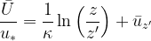
To show the physical significance of the kink, then, McEwan had to do away with the logarithmic velocity profile and replace it with a velocity profile function derived from a hyperbolic-tangent shear distribution. The reason of this choice was pragmatic: firstly, a tanh(z) function arose from a visual curve-fitting exercise to the fluid shear stress distribution predicted by the numerical model of McEwan and Willetts (1991) published two years earlier; secondly, the curve had an asymptotic behavior both near the surface and at the top of the grain layer, and, most importantly, had a point of inflection. Figure 5 shows plots of the derivative of the hyperbolic tangent stress profile proposed by McEwan (1993) in a solid line and the numerical results of McEwan and Willetts (1991) in a dashed line. Derivative d $\displaystyle \tau$ /dz is a measure of force per unit volume; both curves for this derivative, analytical and numerical, indeed have kinks, reaching maxima at z $\displaystyle \approx$ 4.2 mm.

Figure 5. Plot of height from surface versus d $\displaystyle \tau$ /dz, as determined by McEwan’s (1993) hyperbolic tangent shear distribution (solid line) and the numerical model by McEwan and Willetts (1991) (dashed line).

Finally, McEwan (1993) returns to Bagnold’s original explanation of the kink. Bagnold associated the kink with the height at which a characteristic trajectory acquires the bulk of its forward momentum from the wind. In other words, Bagnold associated the kink with a maximum in the force exerted by the grains on the wind. McEwan’s analysis partially confirms this interpretation, noting, however, that the maximum in the force per unit volume profile is not caused by a characteristic trajectory and any attempts to explain the kink in terms of an average trajectory would be misleading.

Bagnold also commented that the kink was less pronounced for well-mixed sands, asserting that this occurred because grains of different sizes have different characteristic trajectories. McEwan noted that, while true, this finding can be restated without any recourse to a characteristic trajectory concept. Willetts and Rice (1985) noted that grains of different sizes tend to rebound from the surface at larger angles, thus the height travelled by grains will be dependent on size. For a well-mixed sand the force per unit volume profile will be a complex product of masses and velocities as a function of height of all the transported grains. Thus, resulting from a wider distribution of rebound angles, there is a wider spectrum of trajectories and hence a less pronounced maximum in the force per unit volume profile, and ultimately a less well-defined kink.

4. Equations of motion for a saltating sand grain (Anderson and Hallet, 1986; White and Schulz, 1977)

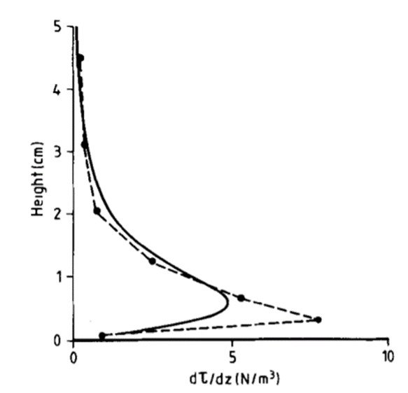
For a more detailed assessment of saltation motion, we must abandon the purely kinematic treatment of a sand particle’s motion presented at the end of section 2 and introduce a dynamic analysis. Most such investigations consider the sand-particle motion to be driven by four forces (Figure 6), namely (1) the particle’s weight, F_g; (2) the aerodynamic drag, F_D; (3) the aerodynamic lift, F_L; and (4) the Magnus lift that results from particle spin, F_M. Each force is briefly discussed below.

Figure 6. Forces acting on a saltating sand grain: (1) weight, F_g; (2) drag, F_D; (3) lift, F_L; (4) Magnus effect lift, F_M.

Particle weight: This force points downward and has intensity equal to the product of the sand grain mass and g = 9.81 m/s². Since the sand grain is immersed in air, a fluid, Archimedes’ principle implies that the weight of the particle should be counteracted by an upward buoyancy force proportional to the volume of fluid displaced by the particle and the density of the fluid. However, the density of air is no greater than 1.2 kg/m³ or so, which is about 2200 times lower than the density of quartz, a typical mineral constituent of sand. Accordingly, we can reasonably neglect buoyancy and assume that F_gis simply the weight of the particle.

Drag: Aerodynamic drag equals the product of drag coefficient, dynamic pressure (= (1/2) $\displaystyle \rho U_{{\text{rel}}}^{2}$ ), and the cross-sectional area of the particle perpendicular to the force vector,

$\displaystyle {{\mathbf{F}}_{D}}={{C}_{d}}\frac{1}{2}\rho {{U}_{{\text{rel}}}}{{\mathbf{U}}_{{rel}}}A$

The relative velocity $\displaystyle {{\mathbf{U}}_{{\text{rel}}}}$ is given by the difference $\displaystyle \mathbf{\bar{U}}$ – $\displaystyle {{\mathbf{U}}_{p}}$ , where $\displaystyle \mathbf{\bar{U}}$ is the mean velocity of the wind and $\displaystyle {{\mathbf{U}}_{p}}$ is the particle velocity. Drag on spherical particles in external flow is a well-known function of particle Reynolds number, as shown, for example, in Chapter 9 of Gerhart et al. (2016).

Lift: Aerodynamic lift arises from shear in the flow that gives rise to a pressure gradient normal to the shear in the direction of increasing velocity. The magnitude of the resulting lift force may be expressed as

$\displaystyle {{F}_{L}}={{C}_{L}}\frac{1}{2}\rho \left( {U_{{\text{top}}}^{2}-U_{{\text{bot}}}^{2}} \right)A$

where $\displaystyle {{U}_{{top}}}$ and $\displaystyle {{U}_{{bot}}}$ are the air speeds at heights corresponding to the top and bottom of the grain, respectively, and C_L is the lift coefficient, which may be taken as 0.85C_d (Chepil, 1958). In general, aerodynamic lift in air will be important only very near the bed, where the velocity gradients are greatest. This assumption, combined with a classic paper’s (Owen (1964)) demonstration that shear throughout the saltation layer is greatly reduced by the grain motion, led several researchers to assume a uniform air velocity within the saltation layer and ignore aerodynamic lift in calculations of saltation trajectory.

Magnus effect: As a grain spins, the air streamlines around the grain become asymmetric. On the underside of the grain, the grain and the air adjacent to it move against the wind direction. On the underside of the grain, the grain and the air adjacent to it move against the wind direction. On the upper side, they move in the same direction as the wind flow. Difference in pressure between the two regions gives rise to a lift-like force known as the Magnus effect. This force is especially significant for grains larger than 0.1 mm in diameter (White and Schulz, 1977). The Magnus lift force on a rotating grain can be estimated as

$\displaystyle {{\mathbf{F}}_{m}}=\frac{{\pi \rho {{d}^{3}}}}{8}\left( {\mathbf{\Omega }\times {{\mathbf{U}}_{{\text{rel}}}}} \right)$

where $\displaystyle \mathbf{\Omega }$ is the angular velocity of the particle, which is taken to be positive for topspin. The angular acceleration of the particle is

$\displaystyle \frac{{d\mathbf{\Omega }}}{{dt}}=\frac{{\pi \mu {{d}^{3}}}}{I}\left( {\frac{1}{2}\frac{{\partial \mathbf{U}}}{{\partial z}}-\mathbf{\Omega }} \right)$

where $\displaystyle \mu$ is the dynamic viscosity of air (= 1.8 $\displaystyle \times$ 10^-5 Pa $\displaystyle \cdot$ s at 15^oC) and I is the mass moment of inertia (= 0.1md² for a spherical grain of mass m). The first term on the right-hand side expresses the acceleration of the spin which results from the difference of the air velocity on opposite sides of the grain, while the second term reflects deceleration which results from the viscosity of the air.

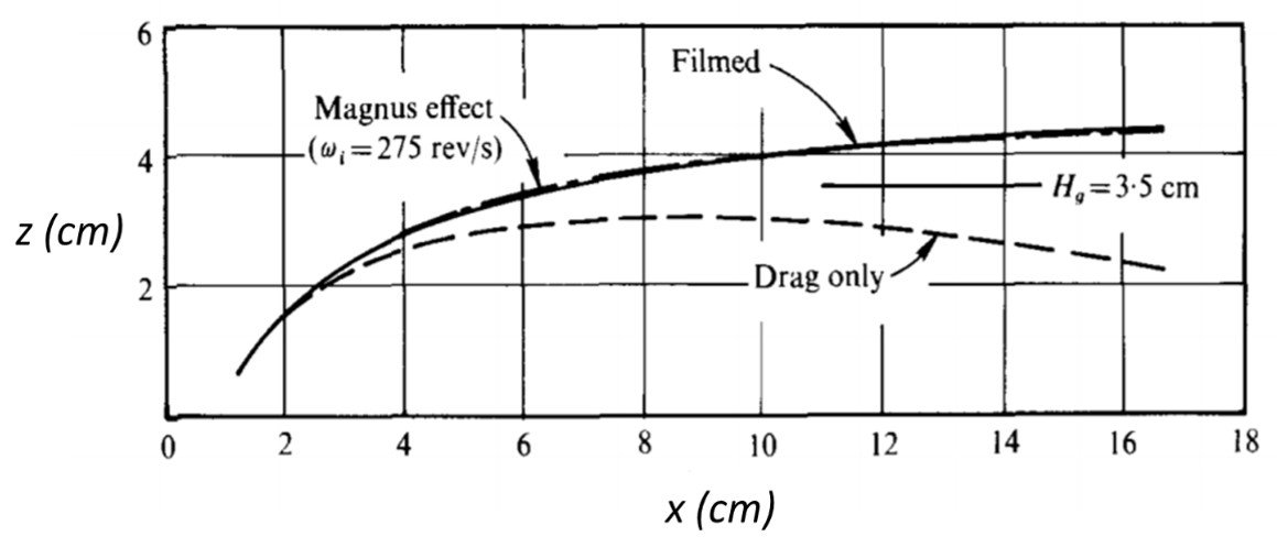
That the Magnus effect is often essential to produce good agreement between theoretical and experimental saltation trajectories has been shown by White and Schulz (1977). Those researchers filmed two-dimensional trajectories of glass spheres in an environmental wind tunnel and plotted the results in an xz plane, as shown in Figure 7. The solid line, labeled Filmed, is a typical saltation trajectory observed in their experiment; the dashed line, labeled Drag only, is the theoretical trajectory predicted with equations of motion that include drag but do not account for the Magnus effect. Clearly, agreement between the two trajectories is poor. Adding a Magnus-lift component with a particle spin rate of 275 rev/s greatly improves the accuracy of the saltation model.

Figure 7. A comparison of a filmed (solid line) path traced out by a particle with theoretical calculations (dashed lines) from the equations of motion with and without a particle spin rate of 275 rev/s. Also shown is the maximum height H_g possible in the absence of all forces except gravity.

The four forces acting on a grain may be decomposed into x (horizontal) and z (vertical) components to yield two equations of motion for a saltating particle through a two-dimensional trajectory. In the x-direction, we have

$\displaystyle m\frac{{\partial U}}{{\partial t}}=\frac{1}{2}\rho {{C}_{d}}A{{U}_{{\text{rel}}}}\left( {\bar{U}-{{U}_{p}}} \right)+\frac{{\pi \rho {{d}^{3}}}}{8}W\Omega$

where W is the vertical velocity of the particle and $\displaystyle \Omega$ is the component of angular velocity perpendicular to the xz plane. In the z-direction, we have

$\displaystyle m\frac{{\partial W}}{{\partial t}}=-mg-\frac{1}{2}\rho {{C}_{d}}A{{U}_{{\text{rel}}}}W+\frac{{\pi \rho {{d}^{3}}}}{8}\left( {\bar{U}-{{U}_{p}}} \right)\Omega +\frac{1}{2}\rho \left( {0.85{{C}_{d}}} \right)A\left( {U_{{\text{top}}}^{2}-U_{{\text{bott}}}^{2}} \right)$

For grains that have topspin ( $\displaystyle \Omega$ > 0), the Magnus force will accelerate the grain upward as long as the horizontal velocity of the grain is less than that of the wind; in the horizontal, the Magnus force will accelerate the grain downwind on the upward limb (W < 0) of the trajectory and decelerate the grain on the descent.

Dividing the two preceding equations through by the mass of the particle gives expressions for the accelerations. To produce a solution, we first specify diameter d, particle density $\displaystyle {{\rho }_{p}}$ , and the wind profile U(z). Then, given a liftoff angle $\displaystyle \alpha$ , a speed of liftoff $\displaystyle {{U}_{{p,0}}}$ , and the initial particle spin in revolutions per second $\displaystyle {{S}_{0}}$ , the initial conditions become

$\displaystyle {{U}_{0}}={{U}_{{p,0}}}\cos \alpha$

$\displaystyle {{W}_{0}}={{U}_{{p,0}}}\sin \alpha$

$\displaystyle {{\Omega }_{0}}=2\pi {{S}_{0}}$

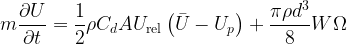
The trajectories calculated by Anderson and Hallet (1986) using the model introduced above agree with preceding calculations by White and Schulz (1977), allowing similar conclusions regarding the importance of the various forces acting on the particle. In the no-spin cases, the maximum trajectory height is consistently 20% to 60% below that estimated if all the initial kinetic potential energy were converted to potential energy (h = $\displaystyle W_{0}^{2}$ /2 $\displaystyle g$ ). As drag in the vertical is roughly proportional to the square of the liftoff velocity, particles ejected at high angles and high speeds will fall shorter of this “no-drag height” than will others (Figure 8).

Figure 8. Hop height relative to $\displaystyle W_{0}^{2}$ /2 $\displaystyle g$ , the height that a particle would reach in an ideal parabolic trajectory, plotted as a function of liftoff velocity. d = 0.25 mm. Labels refer to shear velocities u_*= 0.4, 0.8 m/s.

Typical trajectory durations are on the order of 0.1 – 0.2 sec, and are consistent within 10% of the duration 2W₀/g expected in the absence of nongravitational forces.

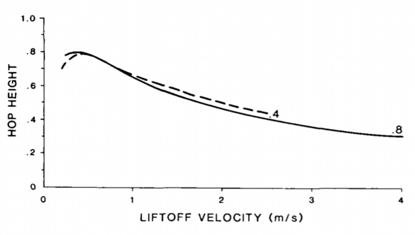
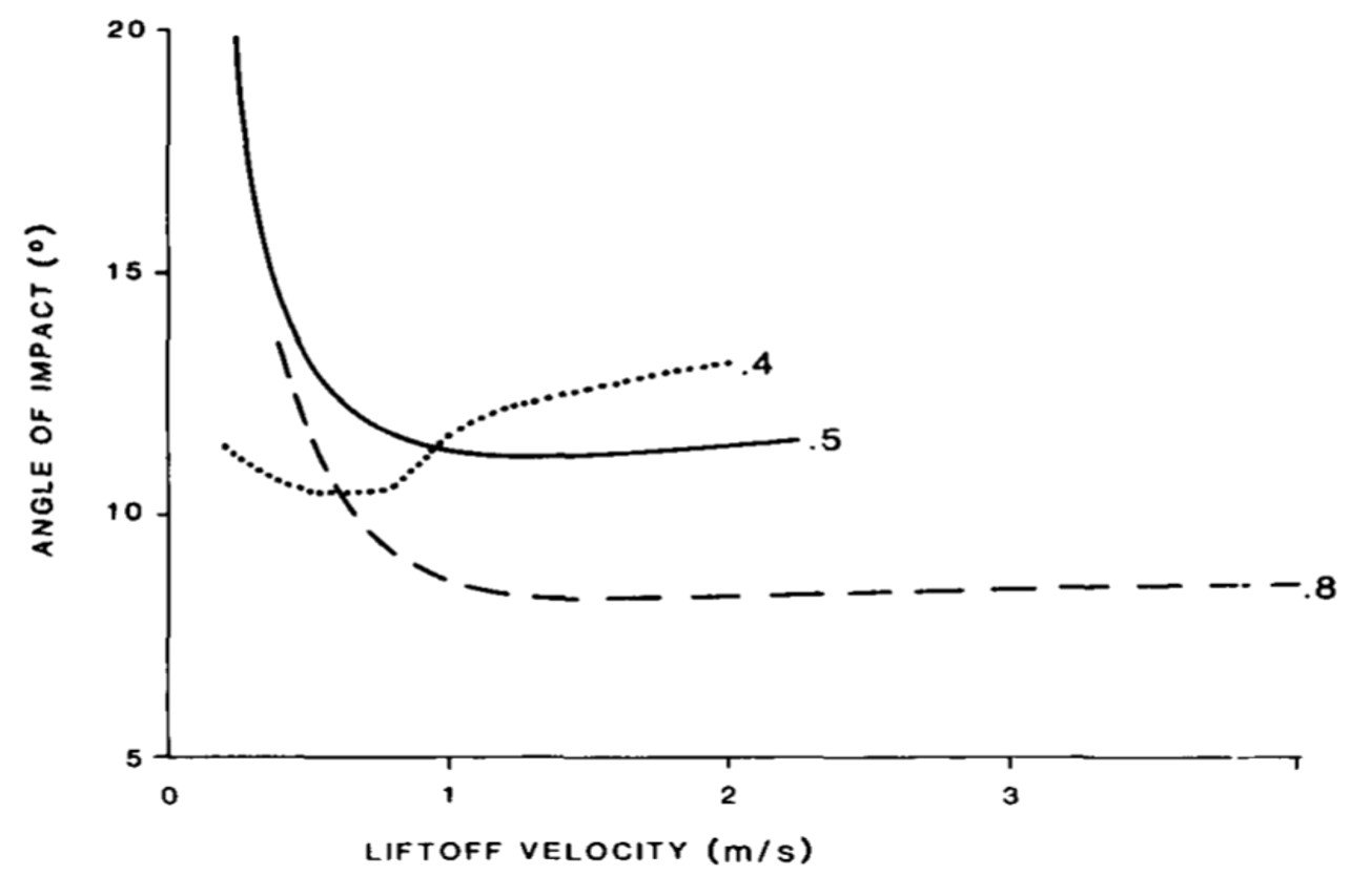
The trajectory length is strongly influenced by the vertical component of the liftoff velocity for a given wind strength (Figure 9). A large range of hop lengths can therefore be expected to result from a realistic range of vertical liftoff speeds, such as that measured by White and Schulz (1977). Hop lengths are remarkably similar for different grain sizes ranging from 0.15 to 0.35 mm that experience identical liftoff conditions. Because drag is inversely related to grain size, smaller grains do not travel as high, but undergo greater horizontal acceleration than do larger grains. Despite the resulting variation in aspect ratios of trajectories with particle size, the impact angles are only weakly dependent on liftoff velocity (Figure 10), in accord with Bagnold’s original observations and with more detailed measurements of impact angle made by White and Schulz (1977).

Figure 9. Hop length as a function of liftoff velocity for u_* = 0.4, 0.5 and 0.8 m/s. d = 0.25 mm, $\displaystyle \alpha$ = 90^o.

Figure 10. Angle of impact with the bed as a function of liftoff velocity for u_* = 0.4, 0.5 and 0.8 m/s. d = 0.25 mm, $\displaystyle \alpha$ = 90^o.

Lastly, particles that are ejected with a wide range of vertical trajectories will impact the surface with 3 to 5 times their initial velocities, or 10 to 20 times their initial kinetic energy. The additional energy will be partitioned between the subsequent or “successive” saltation of the same grain, the ejection of one or more additional grains from the bed, and absorption by friction between grains in the bed. This calculation provides some constraint upon the energy available to fracture grains, resulting in the rounding and frosting of grains and in the production of dust fragments.

5. Intermittent saltation (Stout and Zobeck, 1997)

Most research carried out until recently considered the wind that drives Aeolian transport and the accompanying saltation of sand grains as fundamentally steady, immutable phenomena. However, it goes without saying that these are not steady processes. The intermittent nature of sand transport over short time periods (seconds to minutes) results from the temporal fluctuations of instantaneous wind speed and direction (gustiness) as well as surface conditions (e.g., surface moisture, crust development) that limits the supply of sand grains to the air stream. The intermittency function $\displaystyle \gamma$ is the fraction of time during which saltating particles are detected at a given point during a given time period. For example, $\displaystyle \gamma$ = 0.4 means that saltation activity was detected for 40 percent of the measurement period. Having $\displaystyle \gamma$ = 1 would indicate continuous saltation, whereas $\displaystyle \gamma$ = 0 would indicate no saltation at all in the period of observation. This parameter has been around for a while, but it was not until recently, with the development of digital instrumentation and computerized statistical tools, that its precise quantification became possible.

The specification of intermittency will, to some degree, always reflect some aspect of transport sample rate. The high-frequency (6 kHz) saltation sampling by Ellis (2006) demonstrates that even during so-called equilibrium transport conditions there are short time increments (of the order of 0.01 s) where there are no grains moving past a very small cross-section.

The level of intermittency in the saltation process is governed primarily by whether wind speed fluctuations, characterized by the standard deviation $\displaystyle \sigma$ , span the gap between the mean wind speed $\displaystyle \bar{u}$ and the threshold wind speed $\displaystyle {{u}_{t}}$ , expressed by $\displaystyle \bar{u}$ – $\displaystyle {{u}_{t}}$ . A dimensionless parameter that expresses this relative wind strength may be written as

$\displaystyle s=\frac{{\bar{u}-{{u}_{t}}}}{\sigma }$

To demonstrate the relationship between the relative wind strength, s, and the resulting intermittency function, refer to Figure 11.

Figure 11. Relative wind strength scenarios: (a) s < 0; (b) s > 0; and (c) s = 0.

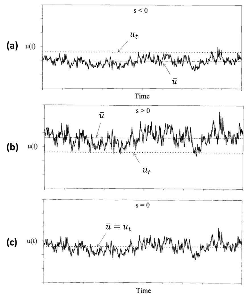
Figure 11a illustrates the condition of a negative relative wind strength, s < 0. If s is negative, then the mean wind speed is less than the threshold value. In this case, occasional gusts may exceed threshold and produce blowing soil. As s $\displaystyle \to$ $\displaystyle -\infty$ , saltation activity tends toward zero, or $\displaystyle \gamma$ $\displaystyle \to$ 0.

Figure 11b illustrates the condition of a positive relative wind strength, s > 0. If s is positive, then the mean wind speed is greater than the threshold value. Under these conditions, saltation will occasionally cease when the wind dips beneath threshold. If s $\displaystyle \gg$ 1, then wind fluctuations $\displaystyle \sigma$ are small compared to the velocity difference $\displaystyle \bar{u}$ – $\displaystyle {{u}_{t}}$ and consequently there is a low probability that winds will dip beneath threshold. As s $\displaystyle \to$ $\displaystyle +\infty$ , soil transport tends toward continuous saltation activity or $\displaystyle \gamma$ $\displaystyle \to$ 1.

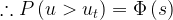
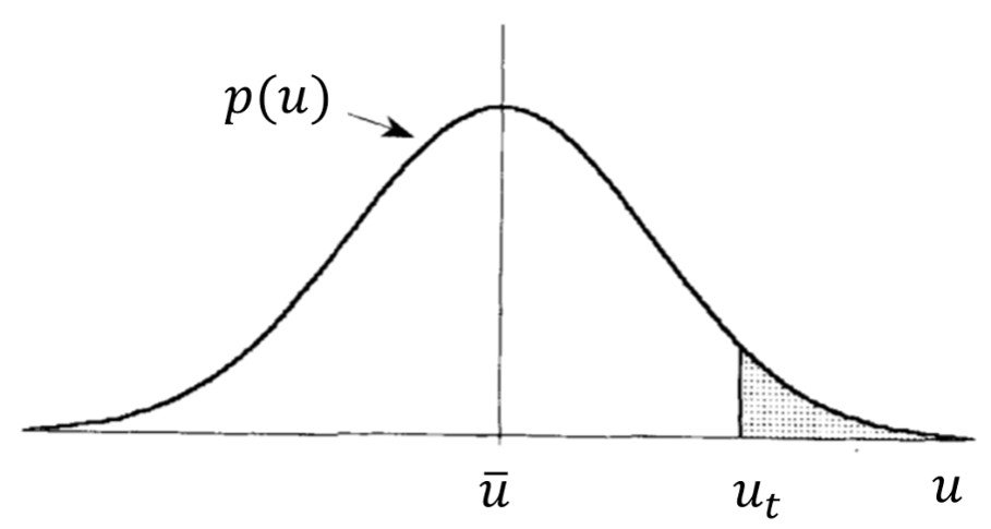
Lastly, Figure 11c illustrates the special case where $\displaystyle \bar{u}$ = $\displaystyle {{u}_{t}}$ and s = 0. In this case, whenever wind fluctuations exceed the mean wind speed, they also exceed threshold.

In turbulent flows, wind speed fluctuations can be described by probability density functions p(u), as depicted schematically in Figure 12. The probability that a given wind speed will exceed threshold is represented by the shaded area beneath the curve in Fig. 12,

$\displaystyle P\left( {u>{{u}_{t}}} \right)=1-\int_{{-\infty }}^{{\frac{{{{u}_{t}}-\bar{u}}}{\sigma }}}{{p\left( q \right)dq}}$

where

$\displaystyle q=\frac{{u-\bar{u}}}{\sigma }$

At this point, we define a distribution function such that

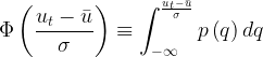
$\displaystyle \Phi \left( {\frac{{{{u}_{t}}-\bar{u}}}{\sigma }} \right)\equiv \int_{{-\infty }}^{{\frac{{{{u}_{t}}-\bar{u}}}{\sigma }}}{{p\left( q \right)dq}}$

The argument within the brackets equals –s, so the probability that the wind speed will exceed threshold may be rewritten in terms of the relative wind strength s as

$\displaystyle P\left( {u>{{u}_{t}}} \right)=1-\Phi \left( {-s} \right)$

However, the PDF in question should satisfy the property

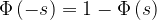
$\displaystyle \Phi \left( {-s} \right)=1-\Phi \left( s \right)$

Combining the two preceding results, we find

$\displaystyle P\left( {u>{{u}_{t}}} \right)=1-\Phi \left( {-s} \right)=1-\left[ {1-\Phi \left( s \right)} \right]$

$\displaystyle \therefore P\left( {u>{{u}_{t}}} \right)=\Phi \left( s \right)$

In mathematical terms, the fraction of time that saltation occurs should equal the fraction of time that winds exceeds threshold. Now, the intermittency function $\displaystyle \gamma$ may be defined as

$\displaystyle \gamma =\Phi \left( s \right)$

This result shows that the intermittency function $\displaystyle \gamma$ follows a curve defined by the distribution function $\displaystyle \Phi$ (s). Stout and Zobeck then proceed to define the form of $\displaystyle \Phi$ (s). This function depends on the relative wind parameter s, which in turn depends on the wind speed distribution. Candidates for wind distribution functions reported in the literature include the normal distribution, the Weibull distribution, and the lognormal distribution.

It is generally agreed that under ideal conditions of homogeneous and stationary turbulence the distribution of a fluid such as wind conforms closely to the normal distribution (see, e.g., Kuo and Corsin, 1971). Although the atmosphere above sandforms is rarely stationary and fully turbulent, Stout and Zobeck quote sources that enable us to consider it a quasi-stationary, turbulent flow. A natural consequence is that the normal distribution may in fact fit a PDF of relative wind strength s.

Figure 12. Schematic drawing of a typical probability density distribution of wind speed. The shaded area represents the probability that the wind speed u is greater than the threshold u_t.

Having completed the theoretical background they needed, Stout and Zobeck went on to report the results of an experimental study they carried out in Lubeck, Texas, to quantify the fraction of time that a given surface experiences saltation and relate saltation activity to wind and surface conditions. Wind speeds were recorded by an anemometer fixed at a height of 2 m in three 1-hour sampling periods, which in turn were divided into 12 5-min periods each. The wind speed distributions in the sampling periods indeed appeared to fit a normal distribution. Most importantly, a plot of intermittency function as a function of relative wind strength s was also well represented by a Gaussian curve, even though Stout and Zobeck could only confirm validity of one half of the curve. In qualitative terms, they showed that during a fairly intense wind erosion event, saltation can be very intermittent, characterized by sporadic bursts of blowing soil that occupy a small fraction of the total time. Saltation activity rarely accounted for more than 50% of any 5-min period and toward the end of the storm, intermittency values often fell below 2%. In short, saltation occupied a small fraction of the total storm period.

References

Download references list here.

Bagnold’s Blown Sand Transport and Saltation

Subscribe to our Mailing List!

Featured Posts

A Primer on NAND Flash Memories

Solidification Time and Chvorinov’s Rule

Step-Growth Polymerization, the Carothers Equation, and the Flory-Schulz Distribution

More Articles

Clairaut’s Theorem and Classical Physical Geodesy

Four Models for One-Dimensional Infiltration of Water in Soils

Fields of Study

More

© 2024 Montogue Quiz

Subscribe to
our Mailing List!

Subscribe to our Mailing List!

Subscribe to receive our latest materials in your inbox.

Homework Help

© 2024 Montogue Quiz

Subscribe to our Mailing List!