River Meandering Models

1. Basic Meander Geometry

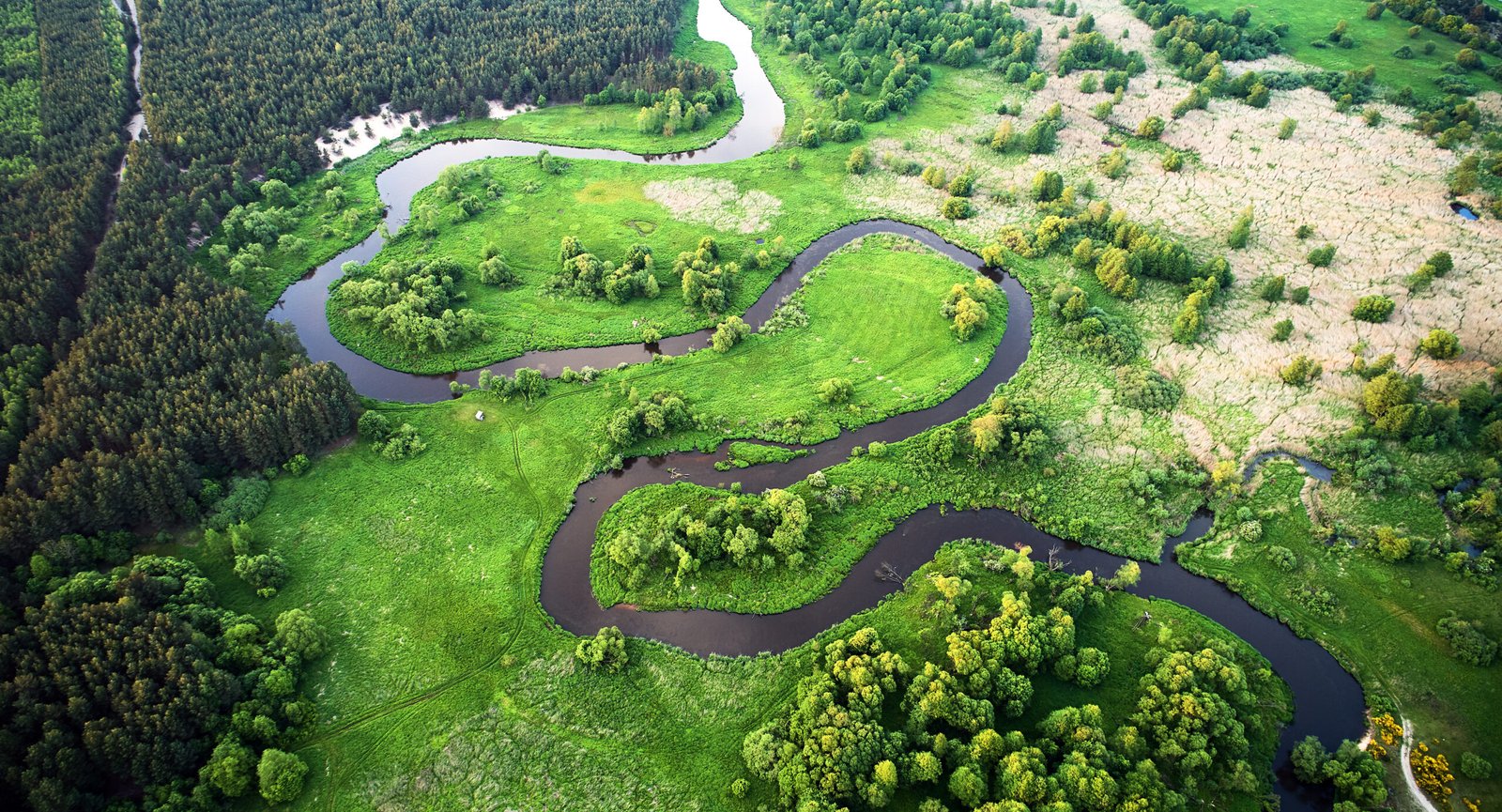
Meandering rivers are characterized by sinuous growth and shift of their courses, a phenomenon known as river migration. This is an evolutionary geomorphic process driven by the interplay of bank erosion and accretion. Sediment is eroded from the eroding banks, usually the outer banks of river bends, and is deposited further downstream near the inner banks. These differential sedimentation processes, coupled with a number of auxiliary effects that we will discuss shortly, lead to the formation of curved shapes. The process is ‘reset’, as it were, when cutoffs occur, leading to the formation of a new reach with its own planimetry and longitudinal slope (Crosato, 2009).

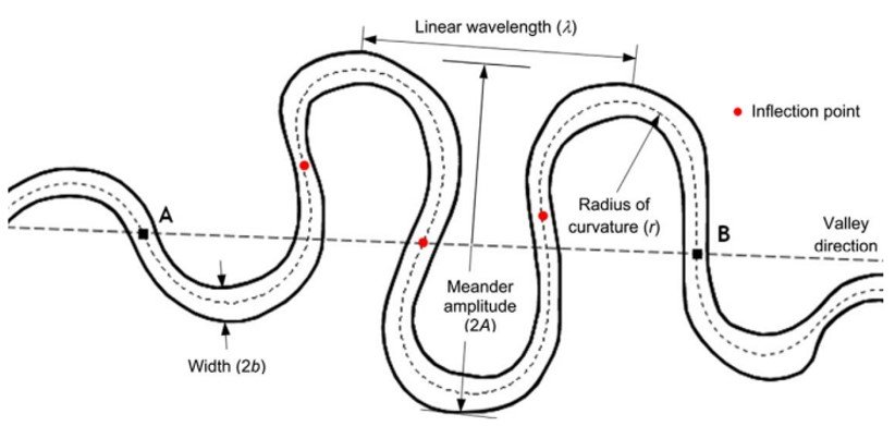
A meander planform is characterized by meander wavelengths $\displaystyle \lambda$ and $\displaystyle {{\lambda }_{c}}$ (i.e., the linear and curvilinear lengths between the apexes or the first inflection points of successive bends on the same side of the river, respectively), meander amplitude 2A, channel width 2b, and radius of curvature R (denoted as r in Figure 1).

Figure 1. A meandering river planform.

When plotting the orientation angle $\displaystyle \theta$ of a river as a function of downstream distance x, Leopold and Langbein (1966) observed that $\displaystyle \theta$ varied as a function of the maximum angle $\displaystyle {{\theta }_{m}}$ set at the origin, the downstream distance x, and the river length L in accordance with the equation

$\displaystyle \theta ={{\theta }_{m}}\cos \left( {\frac{{2\pi x}}{L}} \right)$

The radius of curvature can be obtained by using 1/R = –d $\displaystyle \theta$ /dx, which, referring to the expression above, yields

$\displaystyle \frac{1}{{\left| R \right|}}=\frac{{2\pi {{\theta }_{m}}}}{L}\sin \left( {\frac{{2\pi x}}{L}} \right)$

The river crossing corresponds to x = 0 and R $\displaystyle \to$ $\displaystyle \infty$ . The maximum radius of curvature R_m is obtained at the apex, that is, where x = L/4 and sin(2πx/L) = 1, so that

$\displaystyle {{R}_{m}}=\frac{L}{{2\pi {{\theta }_{m}}}}$

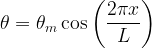
The meander length $\displaystyle \Lambda$ is given by the integral

$\displaystyle \Lambda =\int_{0}^{L}{{\cos \theta dx}}=\int_{0}^{L}{{\cos \left[ {{{\theta }_{m}}\cos \left( {\frac{{2\pi x}}{L}} \right)} \right]dx}}$

$\displaystyle \therefore \Lambda =L{{J}_{0}}\left( {{{\theta }_{m}}} \right)$

where J₀( $\displaystyle {{\theta }_{m}}$ ) is the zero-order Bessel function of the first kind. In a similar manner, the meander width W_m = 2b is expressed as

$\displaystyle {{W}_{m}}=2\int_{0}^{{{L}/{4}\;}}{{\sin \theta dx}}=\int_{0}^{L}{{\sin \left[ {{{\theta }_{m}}\cos \left( {\frac{{2\pi x}}{L}} \right)} \right]dx}}$

$\displaystyle \therefore {{W}_{m}}=\frac{L}{2}{{H}_{0}}\left( {{{\theta }_{m}}} \right)$

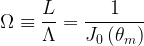
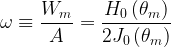
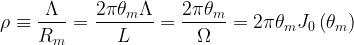
where H₀() is the zero-order Struve function. Following Julien (2018), we note that three main dimensionless quantities describe meandering rivers, namely (1) the sinuosity, $\displaystyle \Omega$ ; (2) the relative meander width, $\displaystyle \omega$ ; and (3) the relative minimum radius of curvature, $\displaystyle \rho$ . These are respectively given by

$\displaystyle \Omega \equiv \frac{L}{\Lambda }=\frac{1}{{{{J}_{0}}\left( {{{\theta }_{m}}} \right)}}$

$\displaystyle \omega \equiv \frac{{{{W}_{m}}}}{A}=\frac{{{{H}_{0}}\left( {{{\theta }_{m}}} \right)}}{{2{{J}_{0}}\left( {{{\theta }_{m}}} \right)}}$

$\displaystyle \rho \equiv \frac{\Lambda }{{{{R}_{m}}}}=\frac{{2\pi {{\theta }_{m}}\Lambda }}{L}=\frac{{2\pi {{\theta }_{m}}}}{\Omega }=2\pi {{\theta }_{m}}{{J}_{0}}\left( {{{\theta }_{m}}} \right)$

Next, we can provide a simple description of the rate of change in the orientation angle for the sine-generated curves that outline the meandering pattern. The time rate of change of $\displaystyle \theta$ is given by

$\displaystyle \dot{\theta }=\frac{{d{{\theta }_{m}}}}{{dt}}=-a\frac{{{{\partial }^{2}}\theta }}{{\partial {{x}^{2}}}}=a{{\left( {\frac{{2\pi }}{\Lambda }} \right)}^{2}}{{\theta }_{m}}J_{0}^{2}\left( {{{\theta }_{m}}} \right)$

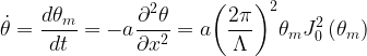
where a is a resistance factor. Separating variables,

$\displaystyle {{t}_{{12}}}=\int_{{{{t}_{1}}}}^{{{{t}_{2}}}}{{dt}}=\frac{1}{a}{{\left( {\frac{\Lambda }{{2\pi }}} \right)}^{2}}\int_{{{{\theta }_{{m1}}}}}^{{{{\theta }_{{m2}}}}}{{\frac{{d{{\theta }_{m}}}}{{{{\theta }_{m}}J_{0}^{2}\left( {{{\theta }_{m}}} \right)}}}}$

where subscripts 1 and 2 refer to the beginning and end of the period of interest, respectively. Let p_c1 denote the mean annual percentage migration rate, which is related to the resistance factor a and the width of the channel by the simple expression a = p_c1W². Further, for a constant $\displaystyle \Lambda$ we may write $\displaystyle \Lambda$ $\displaystyle \approx$ 2 $\displaystyle \pi$ W. Equipped with these relationships, we substitute into the equation above and carry out the integration to obtain

$\displaystyle {{t}_{{12}}}=\frac{1}{{{{p}_{{c1}}}}}\frac{\pi }{2}\left[ {\frac{{{{N}_{0}}\left( {{{\theta }_{{m2}}}} \right)}}{{{{J}_{0}}\left( {{{\theta }_{{m2}}}} \right)}}-\frac{{{{N}_{0}}\left( {{{\theta }_{{m1}}}} \right)}}{{{{J}_{0}}\left( {{{\theta }_{{m1}}}} \right)}}} \right]$

where N₀() is the Neumann function, or the zero-order Bessel Y function. The equation above yields the time required for a channel to increase its deviation angle from $\displaystyle {{\theta }_{{m1}}}$ to $\displaystyle {{\theta }_{{m2}}}$ . Suppose, for instance, that p_ci = 0.05 year^–1, $\displaystyle {{\theta }_{{m1}}}$ = 30^o = 0.524 rad, and $\displaystyle {{\theta }_{{m2}}}$ = 60^o = 1.05 rad; the time required to achieve this change in deviation angle is

$\displaystyle {{t}_{{12}}}=\frac{1}{{0.05}}\times \frac{\pi }{2}\left[ {\frac{{{{N}_{0}}\left( {1.05} \right)}}{{{{J}_{0}}\left( {1.05} \right)}}-\frac{{{{N}_{0}}\left( {0.524} \right)}}{{{{J}_{0}}\left( {0.524} \right)}}} \right]\approx 19.2\,\text{years}$

2. Advanced meandering models

One general characteristic of meandering models is their order, which reflects the number of curvature-related convolution terms in the equations used to formulate the meandering process. A range of linear models with various orders, usually ranging from first to fourth, have been devised since the late 1970s.

The first comprehensive meandering model is that of Ikeda et al. (1981). This approach is based on the following first-order ordinary differential equation:

$\displaystyle \frac{{du}}{{ds}}+2{{\chi }_{1}}u={{\chi }_{1}}{A}'C-\frac{{dC}}{{ds}}$

where u is streamwise velocity; C is the curvature along the streamwise axis s; $\displaystyle {{\chi }_{1}}$ = $\displaystyle \beta$ C₁, where $\displaystyle \beta$ is the width-depth ratio defined as $\displaystyle \beta$ = b/H (where b is one-half the channel width and H is flow depth); and A’ is the scour factor. The solution to this equation links the excess near-bank velocity to the planform curvature and may be written as

$\displaystyle {{u}_{b}}\left( s \right)=-bUC+\frac{{Ub{{C}_{f}}}}{H}\left( {{{F}^{2}}+{A}'+2} \right)\int_{0}^{\infty }{{{{e}^{{{{-2{{C}_{f}}{s}'}}/{H}\;}}}C\left( {s-{s}'} \right)d{s}'}}$

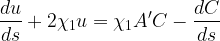
where u_b(s) is excess near-bank velocity along the streamwise axis s, which promotes cutbank erosion; U is the depth-averaged streamwise velocity; C_f = gHI/U² is the friction factor (g is the gravitational acceleration and I is the valley slope); and F is the depth Froude number. Importantly, in the equation above C_f has no spatial variation. Figure 2 shows a sequence of meander evolution obtained with an Ikeda-type model. Although simple, the Ikeda model serves well to model the fundamental characteristics of freely meandering rivers, including phenomena of fattening and upstream skewness of meander bends. Accordingly, the Ikeda model has seen widespread usage in a variety of applications including studies of meander migration, cutoff processes, and the influence of meandering on riparian-vegetation establishment. While it may be adequate before cutoffs occur, the Ikeda model fails to reproduce complex meander forms such as downstream-skewed meanders as well as multilobed meanders and the corresponding irregular planform patterns.

Figure 2. Progression of meanders starting from a sine-generated curve with very small amplitude (Ikeda-type model). From Crosato et al. (2009).

The model proposed by Zolezzi and Seminara (2001) overcomes some of the limitations of the Ikeda model. It uses a linearized formulation for the flow hydrodynamics and bed morphodynamics, but a fully nonlinear formulation for the kinematics of planform evolution. The analytic solution is based on a full coupling between (1) hydrodynamics, sediment transport and bed topography; and (2) curvature-driven secondary currents and topography-driven secondary flow. Further, the model accounts for spatial variation in friction factor and bed-load transport, as well as for vertical variation of eddy viscosity.

Zolezzi and Seminara showed that meandering may be described by a resonance behavior that depends on the channel’s width-to-depth ratio $\displaystyle \beta$ ; specifically, $\displaystyle \beta$ was described by its relationship to a threshold value $\displaystyle {{\beta }_{R}}$ , which characterizes force-free spatial modes of the river system consisting of migrating alternate bars. At this threshold value, the alternate bars can neither grow nor decay in time or space. Simply put, at $\displaystyle \beta$ $\displaystyle \approx$ $\displaystyle {{\beta }_{R}}$ , these modes have no morphodynamic influence on the migrational behavior. The dynamics change, however, as $\displaystyle \beta$ is made less or greater than the threshold value $\displaystyle {{\beta }_{R}}$ , which characterizes sub- and super-resonant conditions, respectively. In streams characterized by sub-resonant conditions (i.e., such that $\displaystyle \beta$ < $\displaystyle {{\beta }_{R}}$ ), the migration rate is influenced by upstream planform morphology, whereas for those characterized by super-resonant conditions (i.e., $\displaystyle \beta$ > $\displaystyle {{\beta }_{R}}$ ), it is influenced by downstream planform morphology. It follows that in contrast to Ikeda’s model, which can only represent upstream-skewed meanders – a setting similar to sub-resonant behavior – the Zolezzi-Seminara model can reliably characterize the evolution of a richer variety of patterns, from simple bends to compound loops to multi-lobed meanders in pre-cutoff timescales.

Frascati and Lanzoni (2009) assessed how much long-term, synthetically generated meandering patterns reproduce the morphological features observed in the field. Howard and Hemberger (1991), using multivariate statistical methods, showed that, despite visual similarities, long-term meander planforms generated by numerical models can be statistically distinguished from natural meanders. As mentioned below, Camporeale et al. (2008) have noted that cutoffs are also associated with a filtering action whereby hydrodynamic effects that are important in the short term may have no effect on the long-term meandering dynamics. In order to investigate this issue, Frascati and Lanzoni combined principal component analysis (PCA) and simulations using both the Ikeda et al. (1981) and the Zolezzi and Seminara (2001) models. They found that only a model that properly resolves both sub-resonant and super-resonant behavior, such as Zolezzi and Seminara’s, can properly reproduce the many bend forms observed in nature not only in short timescales, as in the case typical of evolution of single meanders before cutoff, but also in the long term, when older reaches are removed from the active river by repeated cutoff events.

Perucca et al. (2007) studied the interplay between meandering processes and riparian vegetation. Specifically, Perucca’s team adopted a numerical model with a simple linear link between erodibility coefficient and vegetation biomass. Their simulations highlighted how the variation of erodibility caused by the evolution of riparian biomass influences the shape assumed by the river planform: In view of the continuous river-induced evolution, riparian vegetation develops characteristic biomass density patterns that are able, in turn, to affect river morphology evolution through vegetation-dependent erodibility. This is a complex process of mutual interactions, wherein an important role is played by both the different biomass distributions along the riparian transect and by the temporal scales of growth and decay in vegetation. Perucca’s team found that the planforms obtained while accounting for vegetation-dependent erodibility may be remarkably different from those obtained with constant erodibility; the differences can be of the order of 30% of the meanders’ mean wavelength.

Formation of cutoffs is another phenomenon that contributes substantially to planform evolution in meandering processes. Cutoff is the bypass of a meander loop in favor of a shorter path with the subsequent formation of an abandoned reach, called an oxbow lake. Camporeale et al. (2008) ascribed a dual role for cutoffs in long-term river dynamics. Firstly, cutoff formation functions as a geometrical constraint, limiting the size and development of meanders through the systematic elimination of older reaches in favor of new ones. Secondly, cutoff formation functions as a dynamical process, generating noise that randomly disturbs the deterministic spatiotemporal development of meanders.

In yet another interesting approach, Frascati and Lanzoni (2010) endeavored to find whether the Zolezzi-Seminara model gives rise to chaotic or self-organization behavior. Testing such a behavior with the aid of a numerical model is compulsory because the large time scales associated with meandering preclude a field-based approach. Their results, using a fully nonlinear simulation of the lateral migration of meandering channels and of channel shortening via cutoffs, combined with an analytical description of the linearized flow field, yielded no evidence that long-term meandering dynamics is characterized by the presence of mathematical chaos. Their results corroborate those of Perucca et al. (2005), who had adapted time-series statistical tests with channel coordinate s instead of time values and found that the geometry of the meandering rivers they worked with exhibited no chaotic nonlinearity. Perucca’s team hypothesized that this could be attributable to cutoff dynamics or some sort of stochastic external forcing, which may prevent morphodynamic nonlinearities from developing to a significant extent.

Past work has indicated the occurrence of sharp bends with hydrodynamic behavior markedly different from bends of moderate or mild curvature. Blanckaert (2011) showed that while the width-to-radius of curvature ratio B/R has been widely used to characterize and model meandering processes, it on its own does not accurately parameterize the complex interplay between several hydro- and morphodynamic processes associated with river migration. Blanckaert goes on to note that, as his previous research had showed (Blanckaert and de Vriend, 2003; 2010), an improved formulation can be obtained by complementing B/R with a second parameter $\displaystyle C_{f}^{{-1}}$ H/B, where $\displaystyle {{C}_{f}}$ is the Chézy coefficient and H is the average flow depth. This parameter is representative of a river’s shallowness and roughness. Blanckaert found that reduced meander migration rate and greater meander stability are typical of narrow and relatively deep rivers ( $\displaystyle C_{f}^{{-1}}$ B/H > 10), whereas large shallow rivers ( $\displaystyle C_{f}^{{-1}}$ B/H < 5) exhibit the most dynamic meandering behavior.

3. Numerical Models

Meandering research has also benefitted from several other simulation-driven studies (e.g., Howard, 1983; Sun et al., 1996). In one early example, Sun et al. (1996) combined the Ikeda et al. (1981) approach with a primitive distribution of sedimentary material so as to study the evolution of river geometry in a more accurate manner. Years later, Duan and Julien (2010) used a depth-averaged, two-dimensional model to simulate the hydrodynamic flow field, sediment transport, bank erosion, and ultimately meandering evolution process in a channel shifting from low to high sinuosity. The Duan-Julien model properly simulates the various modes of deformation of meandering channels, including downstream and upstream migration, lateral extension, and rotation of meander bends.

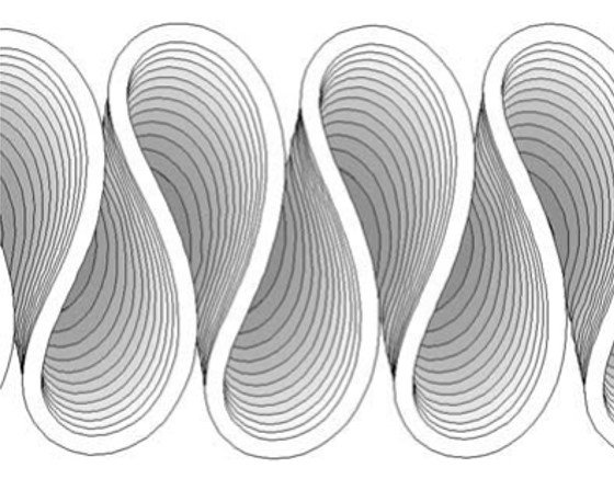
More recently, Asahi et al. (2013) adopted a numerical model that does away with some of the shortcomings of the Duan-Julien simulations, allowing for variations in width, flood effects (modelled through hydrographs) and vegetation dynamics. Figure 3 shows the channel migration and elevation contour patterns for different ratios T_land/T_return; here, T_land denotes the time required for vegetation to become established and T_return denotes the return time of the next flood. It is seen that a shorter time for vegetation to take hold leads to a more sinuous, narrower channel, whereas a time that is so long that it approaches the order of the time between floods leads to a less sinuous, nearly braided channel.

Figure 3. Comparison of channel migration and contour of bed elevation under different conditions depending on the relationship between the parameters T_land and T_return. Case 3 refers to T_land/T_return = 0.025; Case 3-1 refers to T_land/T_return = 0.125; Case 3-2 refers to T_land/T_return = 0.25; Case 3-3 refers to T_land/T_return = 0.5; Case 3-4 refers to T_land/T_return = 1.0. From Asahi et al. (2013).

The assumption of a temporally constant width in a meandering river is partly justified by field observations over geomorphic time, which indicate that several rivers tend to maintain a fairly constant mean channel width as they migrate (as reported, for instance, in Lagasse et al., 2004). However, there is a much heftier body of data indicating that natural rivers undergo time periods of width adjustment as the river responds to changes in flow regime and other environmental factors. Accordingly, workers have recently set about studying river meandering phenomena accompanied by spatial variations in width; the Asahi (2013) study mentioned above is but one prominent example. Using a perturbation method, Luchi et al. (2011) found that meanders with sufficiently intense spatial width variations, and at sufficiently large bankfull aspect ratios, might display a long-term behavior characterized by two different equally unstable planforms instead of the single unstable longitudinal mode that occurs in uniform-width meanders. Of the two ensuing planforms, the one with longer wavelength is close to the most unstable mode with uniform width, while the one with shorter wavelength is associated with complex interactions between curvature and width variations.

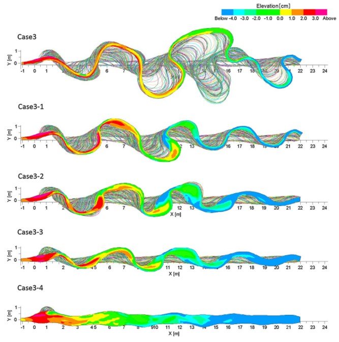
In one of the most sophisticated meandering models produced to date, Eke et al. (2014) studied the coevolution of river planform and width. The model allows for modelling of bank erosion – specifically, it models erosion of purely non-cohesive bank material damped by natural armoring afforded by basal slump blocks. Channel deposition, in turn, is modelled as a function of vegetal encroachment damped by flood flow. The banks are allowed to move independently, so that channel width can vary locally as a result of differential bank migration. Figure 4a shows the centerline migration profile that Eke’s team obtained in an idealized simulation; Figure 4b shows the response of three main variables – half-width $\displaystyle \bar{b}$ , flow depth $\displaystyle {{\bar{H}}_{0}}$ , and slope S₀ – to increasing channel sinuosity; note that as slope reduces, the channel half-width decreases and the flow depth increases.

Those workers also provide a simple comparison of their model to that of Asahi et al. (2013). For one, the two models are similar in their treatments of bank erosion, but bank deposition is treated differently. Further, one immediate advantage of the Eke et al. model is that it was fed and validated with field data from the meandering Pembina River, Canada, whereas the simulations conducted by Asahi et al. were restricted to a generic, experimental scale. The Asahi et al. model also cannot be applied to width evolution in straight reaches, and thus is not yet able to fully describe how average width is maintained in meandering rivers. On the other hand, the Eke et al. model cannot capture the formation and migration of free bars, whereas the Asahi et al. model is not subject to this constraint.

Figure 4. A simulation of the evolution of an idealized periodic channel from an initial low amplitude to high amplitude. (a) Centerline migration over time; (b) Reference channel adjustment over time in response to increasing channel sinuosity. Times T in (a) are in thousands of years. From Eke et al. (2014).

References

Download references list here.

River Meandering Models

Subscribe to our Mailing List!

Featured Posts

A Primer on NAND Flash Memories

Solidification Time and Chvorinov’s Rule

Step-Growth Polymerization, the Carothers Equation, and the Flory-Schulz Distribution

More Articles

Size Reduction, the Three Laws of Comminution, and the Bond Equation

Four Models for One-Dimensional Infiltration of Water in Soils

Fields of Study

More

© 2024 Montogue Quiz

Subscribe to
our Mailing List!

Subscribe to our Mailing List!

Subscribe to receive our latest materials in your inbox.

Homework Help

© 2024 Montogue Quiz

Subscribe to our Mailing List!