A Quick Introduction to Convective Mass Transfer Correlations

In this article, we briefly investigate some of the most common correlations in convective mass transfer.

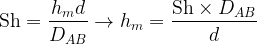
In convective mass transfer, much like in convective heat transfer, systems are modeled by dint of correlations between dimensionless groups. Dimensional analysis reveals that there are three such parameters of interest in typical convection mass transfer problems. The first is the Sherwood number, which can be viewed as a ratio of the intensity of convective mass flux to the intensity of diffusive mass flux, and is mathematically expressed as

$\displaystyle \text{Sh}=\frac{{{{h}_{m}}\times L}}{{{{D}_{{AB}}}}}$

where $\displaystyle {{h}_{m}}$ is the convection mass transfer coefficient, which is analogous to the heat transfer coefficient in Newton’s law of cooling, $\displaystyle {{D}_{{AB}}}$ is the mass diffusivity, and $\displaystyle L$ is a characteristic length of the system being modeled, which may be a diameter (when representing spheres or cylinders), the distance from the leading edge (when representing flat plates), or other representative dimension of the geometry at hand. The second main dimensionless group is the Schmidt number, which is a ratio of the intensity of momentum diffusivity to molecular diffusivity,

$\displaystyle \text{Sc}=\frac{\nu }{{{{D}_{{AB}}}}}$

where, in addition to the Fickian diffusivity, we also have the kinematic viscosity $\displaystyle \nu$ , sometimes called the momentum diffusivity. As the student surely knows, $\displaystyle \nu$ is the ratio of dynamic viscosity to the density of the fluid. The third dimensionless group is the well-known Reynolds number, a ratio of inertial forces to viscous forces,

$\displaystyle Re=\frac{{uL}}{\nu }$

where, besides the characteristic length $\displaystyle L$ and the kinematic viscosity $\displaystyle \nu$ , we also have the flow velocity u. The result of a dimensional analysis of forced convection mass transfer in a simple geometry – say, flow over a flat plate or flow over a sphere – reveals that a valid correlation between the abovementioned parameters has the form

$\displaystyle Sh=f\left( {Re,Sc} \right)$

That is, the Sherwood number is a function of the Reynolds and Schmidt numbers. This is analogous to the general heat transfer functional form

$\displaystyle Nu=f\left( {Re,Pr} \right)$

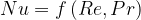
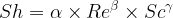
where the Nusselt number substitutes Sh and the Prandtl number takes the place of Sc. The functional form above can be resolved in the general correlation

$\displaystyle Sh=\alpha \times R{{e}^{\beta }}\times S{{c}^{{1/3\ }}}$

where $\displaystyle \alpha$ and $\displaystyle \beta$ are parameters that depend on the geometry being modeled. The fact that $\displaystyle \text{Sh}$ $\displaystyle \propto$ $\displaystyle \text{S}{{\text{c}}^{{{1}/{3}\;}}}$ implicitly implies that the mass transfer coefficient $\displaystyle {{h}_{m}}$ is proportional to the mass diffusivity $\displaystyle {{D}_{{AB}}}$ taken to the 2/3 power, which is consistent with many experimental results. For some situations, $\displaystyle Sc$ $\displaystyle \ne$ 1/3 and we may write a general correlation of the form

$\displaystyle Sh=\alpha \times R{{e}^{\beta }}\times S{{c}^{\gamma }}$

We now present some of the most common forced convection mass transfer correlations, then proceed to three solved examples.

Dittus-Boelter correlations for flow over a flat plate

For laminar flow (Re < $\displaystyle 2\times {{10}^{5}}$ ),

$\displaystyle Sh=0.332Re_{L}^{{1/2\ }}S{{c}^{{1/3\ }}}$

If the mass transfer coefficient used is an averaged quantity, the result above should be doubled, leading to the alternative form

$\displaystyle Sh=\frac{{{{{\bar{h}}}_{m}}L}}{{{{D}_{{AB}}}}}=0.664Re_{L}^{{{1}/{2}\;}}S{{c}^{{1/3\ }}}$

For turbulent flow ( $\displaystyle 5\times {{10}^{5}}$ < Re < $\displaystyle {{10}^{7}}$ ),

$\displaystyle Sh=0.037Re_{L}^{{0.8}}S{{c}^{{1/3\ }}}$

The two foregoing correlations are analogous to the Dittus-Boelter correlation for heat transfer over a flat plate. Since the Dittus-Boelter heat transfer equations are valid for Prandtl numbers greater than 0.6, we may surmise that these analogous mass transfer equations should be valid for Sc > 0.6 only.

Correlations for flow through a circular tube

For laminar flow (Re < 2100),

$\displaystyle Sh=1.62{{\left[ {ReSc\left( {{d}/{L}\;} \right)} \right]}^{{{1}/{3}\;}}}$

where d and L are tube diameter and length, respectively. For turbulent flow in the range 4000 < Re < 60,000 and 0.6 < Sc < 3000, the following correlation is recommended,

$\displaystyle Sh=0.023R{{e}^{{0.83}}}S{{c}^{{1/3\ }}}$

Correlation for forced convection over a cylinder

$\displaystyle Sh=0.3+\frac{{0.62R{{e}^{{1/2\ }}}S{{c}^{{1/3\ }}}}}{{{{{\left[ {1+{{{\left( {0.4/Sc} \right)}}^{{2/3}}}} \right]}}^{{1/4}}}}}{{\left[ {1+{{{\left( {\frac{{Re}}{{282,000}}} \right)}}^{{5/8}}}} \right]}^{{4/5}}}$

Since the corresponding equation for heat transfer is valid for $\displaystyle RePr$ > 0.2, it is reasonable to assume that the analogous mass transfer equation is valid only if $\displaystyle ReSc$ > 0.2.

Froessling correlation for forced convection over a single sphere

$\displaystyle Sh=0.2+0.552R{{e}^{{1/2}}}S{{c}^{{1/3}}}$

We now present three applied examples.

Example 1

Air at 1 atm and 100ºC containing small particles of uranium dioxide is flowing at a velocity of 4 m/s inside a 0.15-m-diameter tube. Calculate the mass transfer coefficient for $\displaystyle U{{O}_{2}}$ , given the kinematic viscosity of air $\displaystyle \nu$ = $\displaystyle 2.32\times {{10}^{{-5}}}$ m²/s and the mass diffusivity $\displaystyle {{D}_{{AB}}}$ = $\displaystyle {4.55\times {{{10}}^{{-8}}}}$ m²/s.

We first determine the Schmidt number,

$\displaystyle \text{Sc}=\frac{\nu }{{{{D}_{{AB}}}}}=\frac{{2.32\times {{{10}}^{{-5}}}}}{{4.55\times {{{10}}^{{-8}}}}}=510$

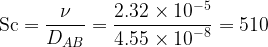
and the Reynolds number,

$\displaystyle Re=\frac{{ud}}{\nu }=\frac{{4\times 0.15}}{{2.32\times {{{10}}^{{-5}}}}}=25,900$

Clearly, Re > 10,000 and the flow is fully turbulent. Since 0.6 $\displaystyle \le$ Sc $\displaystyle \le$ 3000 and 4000 $\displaystyle \le$ Re $\displaystyle \le$ 60,000, the Gilliland correlation for turbulent flow in a circular pipe can be applied. Accordingly,

$\displaystyle Sh=0.023R{{e}^{{0.83}}}S{{c}^{{0.44}}}$

$\displaystyle \therefore Sh=0.023\times {{25,900}^{{0.83}}}\times {{510}^{{0.44}}}=1640$

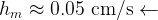
From the definition of Sh, it follows that

$\displaystyle \text{Sh}=\frac{{{{h}_{m}}d}}{{{{D}_{{AB}}}}}\to {{h}_{m}}=\frac{{\text{Sh}\times {{D}_{{AB}}}}}{d}$

$\displaystyle \therefore {{h}_{m}}=\frac{{1640\times \left( {4.55\times {{{10}}^{{-8}}}} \right)}}{{0.15}}=4.97\times {{10}^{{-4}}}\,\text{m/s}$

$\displaystyle {{h}_{m}}\approx 0.05\,\,\text{cm/s}\leftarrow$

Example 2 (Modified from Çengel & Ghajar, 2015)

Consider a 5-m x 5-m wet concrete patio with an average water film thickness of 0.3 mm. Now wind at 50 km/h is blowing at the surface. If the air is at 1 atm, 15ºC, and 35 percent relative humidity, determine how long it will take for the patio to dry completely. The mass diffusivity of water vapor in air at 15ºC may be taken as $\displaystyle 2.33\times {{10}^{{-5}}}$ m²/s, and the saturation pressure of water at the temperature of interest is 1.71 kPa. The density and kinematic viscosity of air at the temperature of interest are 1.225 kg/m³ and $\displaystyle 1.47\times {{10}^{{-5}}}$ m²/s, respectively.

To begin, we determine the Reynolds number of the flow,

$\displaystyle Re=\frac{{uL}}{\nu }=\frac{{\left( {50/3.6} \right)\times 5}}{{1.47\times {{{10}}^{{-5}}}}}=4.72\times {{10}^{6}}$

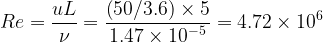
Since Re > 500,000, flow is turbulent over most of the surface. The Schmidt number is

$\displaystyle \text{Sc}=\frac{\nu }{{{{D}_{{AB}}}}}=\frac{{1.47\times {{{10}}^{{-5}}}}}{{2.33\times {{{10}}^{{-5}}}}}=0.631$

and the Sherwood number can be established with the correlation

$\displaystyle \text{Sh}=0.037R{{e}^{{0.8}}}S{{c}^{{{1}/{3}\;}}}$

$\displaystyle \therefore \text{Sh}=0.037\times {{\left( {4.72\times {{{10}}^{6}}} \right)}^{{0.8}}}\times {{0.631}^{{{1}/{3}\;}}}=6930$

Using the definition of Sherwood number, the mass transfer coefficient is determined to be

$\displaystyle {{h}_{m}}=\frac{{\text{Sh}\times {{D}_{{AB}}}}}{L}=\frac{{6930\times \left( {2.33\times {{{10}}^{{-5}}}} \right)}}{5}=0.0323\,\,\text{m/s}$

Observing that the air at the water surface will be saturated and that the saturation pressure of water at 15ºC is 1.71 kPa, the mass fraction of water vapor in the air at the surface and at the free stream conditions are respectively

$\displaystyle {{w}_{{A,s}}}=\frac{{{{P}_{{\text{sat}}}}}}{P}\frac{{{{M}_{A}}}}{{{{M}_{{\text{air}}}}}}=\frac{{1.71}}{{101.325}}\times \frac{{18}}{{29}}=0.0105$

and

$\displaystyle {{w}_{{A,\infty }}}=\frac{{\phi {{P}_{{\text{sat}}}}}}{P}\frac{{{{M}_{A}}}}{{{{M}_{{\text{air}}}}}}=0.35\times \frac{{1.71}}{{101.325}}\times \frac{{18}}{{29}}=0.00367$

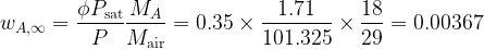
where M_A is the molar mass of water and M_air is the average molar mass of air. The rate of mass transfer to the air is then

$\displaystyle {{\dot{m}}_{{\text{evap}}}}={{h}_{{\text{mass}}}}\rho A\left( {{{w}_{{A,s}}}-{{w}_{{A,\infty }}}} \right)$

$\displaystyle \therefore {{\dot{m}}_{{\text{evap}}}}=0.0323\times 1.225\times \left( {5\times 5} \right)\times \left( {0.0105-0.00367} \right)=0.00676\,\,\text{kg/s}$

The total mass of water in the concrete patio is

$\displaystyle {{m}_{{\text{water}}}}=\rho \forall =1000\times \left[ {5\times 5\times \left( {0.3\times {{{10}}^{{-3}}}} \right)} \right]=7.5\,\,\text{kg}$

Finally, we can divide the mass of water by the evaporation rate and determine the time needed to dry the patio completely,

$\displaystyle \Delta {{t}_{{\text{evap}}}}=\frac{{{{m}_{{\text{water}}}}}}{{{{{\dot{m}}}_{{\text{evap}}}}}}=\frac{{7.5}}{{0.00676}}=1110\,\,\text{s}$

$\displaystyle \Delta {{t}_{{\text{evap}}}}=18.5\,\,\text{min}\leftarrow$

The patio should be completely dry within approximately 19 minutes.

Example 3 (Modified from Dutta, 2007)

A naphthalene ball of 1 cm diameter is suspended in a stream of air flowing at a velocity of 5 m/s at 50ºC and 1 atm total pressure. Calculate the time required for its diameter to be halved. The sublimation pressure of napthalene at the temperature of interest is 0.87 mmHg. The mass diffusivity of naphthalene in air at the temperature of interest is $\displaystyle {{D}_{{AB}}}$ = $\displaystyle 7.3\times {{10}^{{-6}}}$ m²/s and the density of solid naphthalene at 50ºC is $\displaystyle \rho$ = 1130 kg/m³. The density and viscosity of air at the temperature of interest are $\displaystyle \rho$ = 1.09 kg/m³ and $\displaystyle \mu$ = $\displaystyle 1.8\times {{10}^{{-5}}}$ Pa-s, respectively.

The expression to use is the Froessling correlation,

$\displaystyle Sh=2+0.552R{{e}^{{1/2}}}S{{c}^{{1/3\ }}}$

The Reynolds number and therefore the Sherwood number depend upon the radius of the ball, which decreases with time. If r is the radius of the naphthalene ball at any time t, the Reynolds number is

$\displaystyle Re=\frac{{\rho u\left( {2r} \right)}}{\mu }=\frac{{1.09\times 5\times 2}}{{1.8\times {{{10}}^{{-5}}}}}r=6.06\times {{10}^{5}}r$

The maximum value of Re is 3030. The Schmidt number is determined next,

$\displaystyle \text{Sc}=\frac{\mu }{{\rho {{D}_{{AB}}}}}=\frac{{1.8\times {{{10}}^{{-5}}}}}{{1.09\times \left( {7.3\times {{{10}}^{{-6}}}} \right)}}=2.26$

Substituting in the Froessling correlation, we get

$\displaystyle \text{Sh}=2.0+0.552\times {{\left( {\text{6}\text{.06}\times \text{1}{{\text{0}}^{5}}r} \right)}^{{{1}/{2}\;}}}\times \text{2}\text{.2}{{\text{6}}^{{{1}/{3}\;}}}$

$\displaystyle \therefore \text{Sh}=2.0+564{{r}^{{{1}/{2}\;}}}$

The concentration-based mass transfer coefficient is related to the pressure-based mass transfer coefficient by an expression of the form $\displaystyle {{h}_{m}}$ = $\displaystyle {{h}_{{m,P}}}RT$ . From the definition of Sherwood number, we write

$\displaystyle \text{Sh}=\frac{{{{h}_{m}}d}}{{{{D}_{{AB}}}}}=\frac{{{{h}_{{m,P}}}RT\times 2r}}{{{{D}_{{AB}}}}}$

$\displaystyle \therefore \text{Sh}=\frac{{{{h}_{{m,P}}}\times 0.08317\times 323\times 2r}}{{7.3\times {{{10}}^{{-6}}}}}$

$\displaystyle \therefore \text{Sh}=7.36\times {{10}^{6}}r{{h}_{{m,P}}}$

so that

$\displaystyle 7.36\times {{10}^{6}}r{{h}_{{m,P}}}=2.0+564{{r}^{{{1}/{2}\;}}}$

$\displaystyle \therefore {{h}_{{m,P}}}=\frac{{2.0}}{{7.36\times {{{10}}^{6}}r}}+\frac{{564{{r}^{{{1}/{2}\;}}}}}{{7.36\times {{{10}}^{6}}r}}$

$\displaystyle \therefore {{h}_{{m,P}}}=\frac{{2.72\times {{{10}}^{{-7}}}}}{r}+\frac{{7.66\times {{{10}}^{{-5}}}}}{{\sqrt{r}}}$

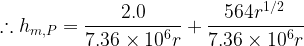
At this point, we relate the rate of change of the ball size with the mass transfer rate. At time t, the rate of sublimation can be expressed as

$\displaystyle -\frac{d}{{dt}}\left( {\frac{4}{3}\pi {{r}^{3}}\frac{\rho }{M}} \right)=\left( {4\pi {{r}^{2}}} \right){{h}_{{m,P}}}\left( {{{P}_{{A,v}}}-{{P}_{{A,\infty }}}} \right)$

$\displaystyle -\frac{{dr}}{{dt}}=\left( {\frac{M}{\rho }} \right){{h}_{{m,P}}}{{P}_{{A,v}}}$

Here, $\displaystyle \rho$ = 1130 kg/m³ is the density of solid naphthalene at 50ºC, $\displaystyle M$ = 128 g/mol is the molar mass of naphthalene, $\displaystyle {{P}_{{A,v}}}$ = 0.87 mmHg = 0.00116 bar is the vapor pressure of naphthalene at 50ºC, and $\displaystyle {{P}_{{A,\infty }}}$ = 0 is the partial pressure of naphthalene in bulk air. Inserting the numerical values in the equation above gives

$\displaystyle -\frac{{dr}}{{dt}}=\frac{{128}}{{1130}}\times \left( {\frac{{2.72\times {{{10}}^{{-7}}}}}{r}+\frac{{7.66\times {{{10}}^{{-5}}}}}{{\sqrt{r}}}} \right)\times 0.00116$

$\displaystyle \therefore -\frac{{dr}}{{dt}}=\frac{{3.57\times {{{10}}^{{-11}}}}}{r}+\frac{{1.01\times {{{10}}^{{-8}}}}}{{\sqrt{r}}}$

Separating variables,

$\displaystyle dt=-\frac{{dr}}{{\frac{{3.57\times {{{10}}^{{-11}}}}}{r}+\frac{{1.01\times {{{10}}^{{-8}}}}}{{\sqrt{r}}}}}$

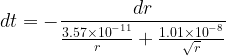
The required time follows if we integrate from the initial radius $\displaystyle {{r}_{0}}$ = 0.5 cm to the final radius $\displaystyle {{r}_{f}}$ = 0.25 cm, that is,

$\displaystyle t=-\int_{{0.005}}^{{0.0025}}{{\frac{{dr}}{{\frac{{3.57\times {{{10}}^{{-11}}}}}{r}+\frac{{1.01\times {{{10}}^{{-8}}}}}{{\sqrt{r}}}}}}}$

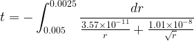
The integral on the right-hand side can be evaluated with the simple Mathematica code

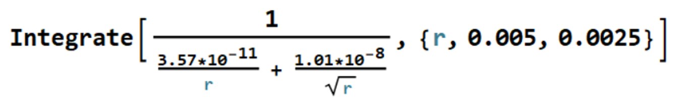
which returns -14,300 sec, so that

$\displaystyle t=-\left( {-14,300} \right)=14,300\,\,\sec =3.97\,\,\text{h}\leftarrow$

The naphthalene ball should require approximately four hours to have its diameter halved.

Go further

Montogue also offers a free quiz on mass transfer by diffusion, which can be found here. Since convection mass transfer is analogous to convective heat transfer, students would do well to check out our free materials on internal convection, external convection, and natural convection. Enjoy!

References

• ÇENGEL, Y. and GHAJAR, A. (2015). Heat and Mass Transfer: Fundamentals and Applications. 5th edition. New York: McGraw-Hill.

• DUTTA, B. (2007). Principles of Mass Transfer and Separation Processes. New Delhi: PHI Learning.

• KESSLER, D. and GREENKORN, R. (1999). Momentum, Heat, and Mass Transfer Fundamentals. New York: Marcel Dekker.

A Quick Introduction to Convective Mass Transfer Correlations

Subscribe to our Mailing List!

Featured Posts

A Primer on NAND Flash Memories

Solidification Time and Chvorinov’s Rule

Step-Growth Polymerization, the Carothers Equation, and the Flory-Schulz Distribution

More Articles

Plasticity: Tresca and von Mises Yield Criteria

Cruise Flight Performance of Piston-Prop Aircraft

Fields of Study

More

© 2024 Montogue Quiz

Subscribe to
our Mailing List!

Subscribe to our Mailing List!

Subscribe to receive our latest materials in your inbox.

Homework Help

© 2024 Montogue Quiz

Subscribe to our Mailing List!