Estimating Ship Resistance with the Froude and ITTC1957 methods

In this article, we briefly introduce two of the most widely used methods for estimation of ship hydrodynamic resistance: Froude’s method and the 1957 International Towing Tank Conference (ITTC) method.

1. Froude’s method

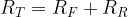
In Froude’s formulation of ship resistance, the total resistance is divided into two components: the frictional resistance, $\displaystyle {{R}_{F}}$ , and the residual resistance, $\displaystyle {{R}_{R}}$ . In mathematical terms,

$\displaystyle {{R}_{T}}={{R}_{F}}+{{R}_{R}}$

The ship resistance estimation process goes as follows. To begin, a geometrically similar model of the full-sized ship is prepared and towed to give its total resistance $\displaystyle {{R}_{{Tm}}}$ . Then, the frictional resistance of the model is computed with Froude’s formula,

$\displaystyle {{R}_{{Fm}}}={{f}_{m}}{{S}_{m}}V_{m}^{n}$

where $\displaystyle {{f}_{m}}$ is a friction factor, $\displaystyle {{S}_{m}}$ is the wetted surface area of the model, $\displaystyle {{V}_{m}}$ is the model speed, and n is an exponent usually taken as 1.825. Having obtained the total resistance and the frictional resistance, the residual resistance can be obtained by subtracting the latter from the former. Next, the model residual resistance is scaled up with the similarity formula

$\displaystyle {{R}_{{RS}}}=\frac{{{{\Delta }_{S}}}}{{{{\Delta }_{m}}}}\times {{R}_{{Rm}}}$

where $\displaystyle {{\Delta }_{S}}$ and $\displaystyle {{\Delta }_{m}}$ are the displacements of ship and model, respectively. Then, the frictional resistance of the ship is estimated, again by dint of Froude’s formula,

$\displaystyle {{R}_{{FS}}}={{f}_{S}}{{S}_{S}}V_{S}^{n}$

where each term has the same meaning as the formula used to determine $\displaystyle {{R}_{{Fm}}}$ . Having determined the frictional and residual resistances for the ship, the results are added to yield the total resistance,

$\displaystyle {{R}_{{TS}}}={{R}_{{FS}}}+{{R}_{{RS}}}$

Equipped with $\displaystyle {{R}_{{TS}}}$ , we can determine the ship effective power by multiplying $\displaystyle {{R}_{{TS}}}$ by the ship velocity, $\displaystyle {{V}_{S}}$ . The following example illustrates the use of Froude’s method.

Example 1

A 5-m long, 224-kg model of a ship is tested at a speed of 2 m/s in a towing tank. At this speed, the total measured resistance of the model is 94 N. The f coefficient for the model is 1.714. The wetted surface area of the model is 7 m². Determine the effective power of the full ship, which has length 125 m, a displacement of 5000 tonnes, a wetted surface area of 4800 m², and a f coefficient equal to 1.551.

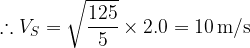
The first step is to determine the speed of the ship; since the Froude numbers are the same for model and ship, we have

$\displaystyle \frac{{{{V}_{M}}}}{{\sqrt{{g{{L}_{M}}}}}}=\frac{{{{V}_{S}}}}{{\sqrt{{g{{L}_{S}}}}}}\to {{V}_{S}}=\sqrt{{\frac{{{{L}_{S}}}}{{{{L}_{M}}}}}}{{V}_{M}}$

$\displaystyle \therefore {{V}_{S}}=\sqrt{{\frac{{125}}{5}}}\times 2.0=10\,\text{m/s}$

The frictional resistance of the model follows from Froude’s formula,

$\displaystyle {{R}_{{Fm}}}={{f}_{m}}{{S}_{m}}V_{m}^{{1.825}}=1.714\times 7.0\times {{2.0}^{{1.825}}}=42.5\,\,\text{N}$

Once the frictional resistance has been determined, we can easily compute the residual resistance of the model,

$\displaystyle {{R}_{{Tm}}}={{R}_{{Fm}}}+{{R}_{{Rm}}}\to {{R}_{{Rm}}}={{R}_{{Tm}}}-{{R}_{{Fm}}}$

$\displaystyle \therefore {{R}_{{Rm}}}=94-42.5=51.5\,\,\text{N}$

Next, we scale up the residual resistance to the full ship using the ratio of displacements,

$\displaystyle \frac{{{{R}_{{RS}}}}}{{{{R}_{{Rm}}}}}=\frac{{{{\Delta }_{S}}}}{{{{\Delta }_{m}}}}\to {{R}_{{RS}}}=\frac{{{{\Delta }_{S}}}}{{{{\Delta }_{m}}}}\times {{R}_{{Rm}}}$

$\displaystyle \therefore {{R}_{{RS}}}=\frac{{5000}}{{0.224}}\times 51.5=1.15\times {{10}^{6}}\,\text{N}$

The frictional resistance of the ship is determined next,

$\displaystyle {{R}_{{FS}}}={{f}_{S}}{{S}_{S}}V_{S}^{{1.825}}=1.551\times 4800\times {{10}^{{1.825}}}=4.98\times {{10}^{5}}\,\text{N}$

Then, we can add the two previous results to establish the total resistance of the ship,

$\displaystyle {{R}_{{TS}}}={{R}_{{RS}}}+{{R}_{{FS}}}$

$\displaystyle \therefore {{R}_{{TS}}}=1,150,000+498,000=1.65\,\,\text{MN}$

Lastly, the ship effective power is found as

$\displaystyle {{P}_{E}}={{R}_{{TS}}}\times {{V}_{S}}=\left( {1.65\times {{{10}}^{6}}} \right)\times 10=16.5\times {{10}^{6}}=16.5\,\ \text{MW}\leftarrow$

2. The 1957 ITTC and the issue of frictional resistance

The ITTC method maintains the essence of Froude’s approach by splitting the resistance coefficient into two components, but incorporates developments of modern fluid dynamics that were not available at the time of Froude’s work. For one, the generic coefficients obtained in Froude’s analysis were replaced with parameters based on dimensional analysis, which have the general form

$\displaystyle \text{Coefficient}=\frac{{\text{Resistance}}}{{\frac{1}{2}\rho S{{V}^{2}}}}$

where $\displaystyle \rho$ is fluid density, $\displaystyle S$ is wetted surface area, and $\displaystyle V$ is velocity. The term (1/2) $\displaystyle \rho {{V}^{2}}$ in the denominator has units of pressure and in fact is sometimes called the dynamic pressure. Multiplying this pressure by the wetted surface area S gives a force; dividing the resistance component in the numerator by this force gives a dimensionless quantity.

The greatest departure of the ITTC method from Froude’s resistance theory, however, has to do with the treatment of frictional resistance. The ITTC approach does away with Froude’s resistance formula and the f frictional coefficient, a parameter that is quite difficult to measure in practice – especially in the case of the full-scale ship – and has little physical meaning. Instead, the 1957 ITTC adopted a frictional resistance modeling approach based on developments of fluid dynamics achieved in the first half of the 20th century, as briefly outlined below (Molland, 2011).

In the 1920s, the legendary aerodynamicist Theodore von Kármán deduced a friction law for flat plates based on a two-dimensional analysis of turbulent boundary layers. The ‘smooth turbulent’ friction law derived by him had the form

$\displaystyle \frac{1}{{\sqrt{{{{C}_{F}}}}}}=A+B{{\log }_{{10}}}\left( {Re\times {{C}_{F}}} \right)$

where $\displaystyle {{C}_{F}}$ is the frictional coefficient, $\displaystyle {Re}$ is the Reynolds number, and A and B are two undetermined constants. In the early 1930s, K.E. Schoenherr replotted all the available experimental data from plank experiments in air and water and attempted to fit this information to von Kármán’s law. The expression he produced was

$\displaystyle \frac{1}{{\sqrt{{{{C}_{F}}}}}}=4.13{{\log }_{{10}}}\left( {Re\times {{C}_{F}}} \right)$

This expression is based on data with significant scatter, but nevertheless constitutes an improvement relatively to Froude’s frictional resistance formula because of the theoretical background that underpins it. The Schoenherr line was adopted by the American Towing Tank Conference in 1947.

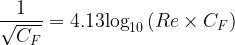
The Schoenherr formula is not very convenient to use because $\displaystyle {{C}_{F}}$ is not explicitly defined for a given $\displaystyle Re$ . The formula can be expanded to give

$\displaystyle \frac{1}{{\sqrt{{{{C}_{F}}}}}}=4.13{{\log }_{{10}}}\left( {Re\times {{C}_{F}}} \right)=4.13\left( {{{{\log }}_{{10}}}Re+{{{\log }}_{{10}}}{{C}_{F}}} \right)$

Since $\displaystyle {{C}_{F}}$ and log $\displaystyle {{C}_{F}}$ vary slowly when compared to Reynolds number, a reasonable approximation to the relation above is

$\displaystyle \frac{1}{{\sqrt{{{{C}_{F}}}}}}=A\left( {{{{\log }}_{{10}}}Re-B} \right)$

where A and B are constants. With B assumed as 2, we can solve for $\displaystyle {{C}_{F}}$ and write

$\displaystyle {{C}_{F}}=\frac{{{A}'}}{{{{{\left( {\text{lo}{{\text{g}}_{{10}}}Re-2} \right)}}^{2}}}}$

where A’ is a modified constant. In 1957, the ITTC adopted a variation of the formula above for use as a ‘correlation line’ in powering calculations. It is termed the ‘ITTC1957 model-ship correlation line’, and closely resembles a formulation proposed by G. Hughes three years earlier:

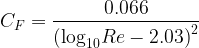
$\displaystyle {{C}_{F}}=\frac{{0.066}}{{{{{\left( {{{{\log }}_{{10}}}Re-2.03} \right)}}^{2}}}}$

The formula adopted by the ITTC rounds 2.03 down to 2.0 and adds a 12% form effect to give

$\displaystyle {{C}_{F}}=\frac{{0.075}}{{{{{\left( {{{{\log }}_{{10}}}Re-2} \right)}}^{2}}}}$

This is the frictional resistance coefficient equation adopted by the 1957 ITTC.

3. Estimating resistance with the Hughes/ITTC1957 method

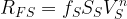
In the ITTC1957 resistance calculation approach, the total resistance coefficient is given by

$\displaystyle {{C}_{T}}=\left( {1+k} \right){{C}_{F}}+{{C}_{W}}$

where (1 + k) is the form factor, $\displaystyle {{C}_{F}}$ is the frictional resistance coefficient, and $\displaystyle {{C}_{W}}$ is the wave-making resistance coefficient. As the name implies, the latter is designated to represent the hydrodynamic resistance caused by flow of waves on the ship hull. Since it is essentially dependent on Froude number – much like frictional resistance depends on Reynolds number – we assume that, in view of Froude number similarity, the value of $\displaystyle {{C}_{W}}$ is the same for model and ship.

The form factor (1 + k) models the influence of hull form on frictional resistance. The factor (1 + k) is incorporated in the so-called viscous coefficient, $\displaystyle {{C}_{V}}$ , which takes account of both skin friction and viscous pressure resistance, so we may write

$\displaystyle {{C}_{T}}=\left( {1+k} \right){{C}_{F}}+{{C}_{W}}={{C}_{V}}+{{C}_{W}}$

We close this article with two applied examples. Example 2 illustrates use of the modern dimensionless coefficients and the ITTC1957 model-ship correlation line, but retains the Froude terminology and does not include a form factor. Example 3 uses the contemporary terminology and includes a form factor.

Example 2

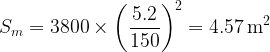
Consider a 150-m long ship with a wetted surface area of 3800 m² and a design speed of 12 knots. Tests on a 5.2-m long geometrically similar model, run at a corresponding speed, gave a total resistance of 40 N in fresh water. Determine the effective power of the full-sized ship. For convenience, take density $\displaystyle \rho$ = 1000 kg/m³ and kinematic viscosity $\displaystyle \nu$ = 1.1 $\displaystyle \times$ 10^-6 m²/s for both model and ship.

From similarity of Froude numbers, we can determine the speed of the model:

$\displaystyle \frac{{{{V}_{m}}}}{{\sqrt{{g{{L}_{m}}}}}}=\frac{{{{V}_{S}}}}{{\sqrt{{g{{L}_{S}}}}}}\to {{V}_{m}}=\sqrt{{\frac{{{{L}_{m}}}}{{{{L}_{S}}}}}}{{V}_{S}}$

$\displaystyle \therefore {{V}_{m}}=\sqrt{{\frac{{5.2}}{{150}}}}\times 12=2.23\,\text{knots}=1.15\,\text{m/s}$

From geometric similarity between ship and model, we can establish the wetted surface area of the model,

$\displaystyle {{S}_{m}}=3800\times {{\left( {\frac{{5.2}}{{150}}} \right)}^{2}}=4.57\,{{\text{m}}^{2}}$

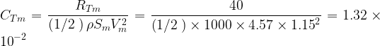
Given the total resistance $\displaystyle {{R}_{{Tm}}}$ = 40 N, we compute the total resistance coefficient for the model,

$\displaystyle {{C}_{{Tm}}}=\frac{{{{R}_{{Tm}}}}}{{\left( {{1}/{2}\;} \right)\rho {{S}_{m}}V_{m}^{2}}}=\frac{{40}}{{\left( {{1}/{2}\;} \right)\times 1000\times 4.57\times {{{1.15}}^{2}}}}=1.32\times {{10}^{{-2}}}$

The model Reynolds number is determined next,

$\displaystyle R{{e}_{m}}=\frac{{{{V}_{m}}{{L}_{m}}}}{\nu }=\frac{{1.15\times 5.2}}{{1.1\times {{{10}}^{{-6}}}}}=5.44\times {{10}^{6}}$

The model frictional coefficient is then

$\displaystyle {{C}_{{Fm}}}=\frac{{0.075}}{{{{{\left( {\log R{{e}_{m}}-2} \right)}}^{2}}}}=\frac{{0.075}}{{{{{\left[ {\log \left( {5.44\times {{{10}}^{6}}} \right)-2} \right]}}^{2}}}}=3.34\times {{10}^{{-3}}}$

The model residual resistance coefficient is obtained by subtracting $\displaystyle {{C}_{{Fm}}}$ from $\displaystyle {{C}_{{Tm}}}$ ,

$\displaystyle {{C}_{{Tm}}}={{C}_{{Fm}}}+{{C}_{{Rm}}}\to {{C}_{{Rm}}}={{C}_{{Tm}}}-{{C}_{{Fm}}}$

$\displaystyle \therefore {{C}_{{Rm}}}=1.32\times {{10}^{{-2}}}-3.34\times {{10}^{{-3}}}=9.86\times {{10}^{{-3}}}$

Now, the Reynolds number for the full ship is

$\displaystyle R{{e}_{S}}=\frac{{{{V}_{S}}{{L}_{S}}}}{\nu }=\frac{{\left( {12\times 0.5144} \right)\times 150}}{{1.1\times {{{10}}^{{-6}}}}}=8.42\times {{10}^{8}}$

and the frictional coefficient is determined as

$\displaystyle {{C}_{{FS}}}=\frac{{0.075}}{{{{{\left( {\log R{{e}_{S}}-2} \right)}}^{2}}}}=\frac{{0.075}}{{{{{\left[ {\log \left( {8.42\times {{{10}}^{8}}} \right)-2} \right]}}^{2}}}}=1.56\times {{10}^{{-3}}}$

The residual resistance coefficient is the same for model and ship; in mathematical terms,

$\displaystyle {{C}_{{RS}}}={{C}_{{Rm}}}=9.86\times {{10}^{{-3}}}$

Gleaning the two previous results, we get the following total resistance coefficient,

$\displaystyle {{C}_{{TS}}}={{C}_{{FS}}}+{{C}_{{RS}}}=\left( {1.56+9.86} \right)\times {{10}^{{-3}}}=1.14\times {{10}^{{-2}}}$

We now have all the information needed to compute the total resistance on the ship.

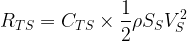
$\displaystyle {{R}_{{TS}}}={{C}_{{TS}}}\times \frac{1}{2}\rho {{S}_{S}}V_{S}^{2}$

$\displaystyle \therefore {{R}_{{TS}}}=\left( {1.14\times {{{10}}^{{-2}}}} \right)\times \frac{1}{2}\times 1000\times 3800\times {{\left( {12\times 0.5144} \right)}^{2}}=825\,\,\text{kN}$

Finally, the ship effective power is

$\displaystyle {{P}_{E}}={{R}_{{TS}}}\times {{V}_{S}}=825,000\times \left( {12\times 0.5144} \right)=5.09\,\text{MW}\leftarrow$

Example 3

What would the effective power be if the ship introduced in the previous problem had a form factor of 1.5?

The total resistance coefficient, Reynolds number, and frictional resistance coefficient for the model remain unchanged. The viscous resistance coefficient for the model is determined as

$\displaystyle {{C}_{{Vm}}}=\left( {1+k} \right){{C}_{{Fm}}}=1.5\times \left( {3.34\times {{{10}}^{{-3}}}} \right)=5.01\times {{10}^{{-3}}}$

The wave-making resistance coefficient, in turn, is given by

$\displaystyle {{C}_{{Wm}}}={{C}_{{Tm}}}-{{C}_{{Vm}}}=1.32\times {{10}^{{-2}}}-5.01\times {{10}^{{-3}}}=8.19\times {{10}^{{-3}}}$

The Reynolds number and frictional resistance coefficient of the ship are also unaltered. The viscous resistance coefficient of the full-sized ship is then

$\displaystyle {{C}_{{VS}}}=\left( {1+k} \right){{C}_{{FS}}}=1.5\times \left( {1.56\times {{{10}}^{{-3}}}} \right)=2.34\times {{10}^{{-3}}}$

The wave-making resistance coefficient of the full-scale ship is the same as that of the model; that is,

$\displaystyle {{C}_{{WS}}}={{C}_{{Wm}}}=8.19\times {{10}^{{-3}}}$

Gathering the two foregoing results, the total resistance coefficient of the ship is

$\displaystyle {{C}_{{TS}}}={{C}_{{VS}}}+{{C}_{{WS}}}=\left( {2.34+8.19} \right)\times {{10}^{{-3}}}=1.05\times {{10}^{{-2}}}$

The total resistance follows as

$\displaystyle {{R}_{{TS}}}={{C}_{{TS}}}\times \frac{1}{2}\rho {{S}_{S}}V_{S}^{2}$

$\displaystyle \therefore {{R}_{{TS}}}=\left( {1.05\times {{{10}}^{{-2}}}} \right)\times \frac{1}{2}\times 1000\times 3800\times {{\left( {12\times 0.5144} \right)}^{2}}=760\,\,\text{kN}$

Lastly, the ship effective power is determined to be

$\displaystyle {{P}_{E}}={{R}_{{TS}}}\times {{V}_{S}}=760,000\times \left( {12\times 0.5144} \right)=4.69\,\,\text{MW}\leftarrow$

That is, inclusion of the form factor leads to an 8% drop in ship effective power.

Limitations

It goes without saying that the treatment presented in this article is an oversimplification of the ship resistance estimation problem. For one, it should be realized that ship hull roughness also contributes to resistance, and is often incorporated in calculations by an additional allowance $\displaystyle \Delta {{C}_{F}}$ on the frictional resistance coefficient. In addition, friction and wave-making are not the only sources of ship drag, as flow of air on the superstructure and the presence of appendages may also contribute substantially to overall resistance. Harvald (1983) and more recently Molland et al. (2011) offer excellent discussions on these and other topics not covered here.

References

• HARVALD, S. (1983). Resistance and Propulsion of Ships. Hoboken: John Wiley and Sons.

• MOLLAND, A., TURNOCK, S., and HUDSON, D. (2011). Ship Resistance and Propulsion. Cambridge: Cambridge University Press.

• PATTERSON, C. and RIDLEY, J. (2014). Ship Stability, Powering and Resistance. London: Bloomsbury.

• TUPPER, E. (2013). Introduction to Naval Architecture. 5th edition. Oxford: Butterworth-Heinemann.

Estimating Ship Resistance with the Froude and ITTC1957 methods

Subscribe to our Mailing List!

Featured Posts

A Primer on NAND Flash Memories

Solidification Time and Chvorinov’s Rule

Step-Growth Polymerization, the Carothers Equation, and the Flory-Schulz Distribution

More Articles

Murray’s Law and the Analysis of Arterial Bifurcations

Plasticity: Tresca and von Mises Yield Criteria

Fields of Study

More

© 2024 Montogue Quiz

Subscribe to
our Mailing List!

Subscribe to our Mailing List!

Subscribe to receive our latest materials in your inbox.

Homework Help

© 2024 Montogue Quiz

Subscribe to our Mailing List!