


1. Introduction
Every transport phenomena course covers internal flow in circular tubes with some depth. Most students are familiar with the Hagen-Poiseuille model, which describes steady, fully-developed flow in a conduit of circular cross-section. The HP model tells us that the velocity distribution in such a conduit is described by the expression

where r is radial distance from the centerline, a is the radius of the cylinder, 

This result is sometimes known as the Poiseuille equation. The velocity profile (1) and the flow rate (2) provide a full description of an internal flow. In this post, we move one step further and consider internal flow in noncircular cross-sectional geometries.
2. Noncircular ducts and the hydraulic diameter
The literature contains several interesting solutions for fully developed laminar flow in ducts of noncircular cross-section. Some of these are summarized in Table 1, following White (2004) and Panton (2013).
Table 1. Velocity profile and flow rate for steady laminar flow in noncircular ducts.
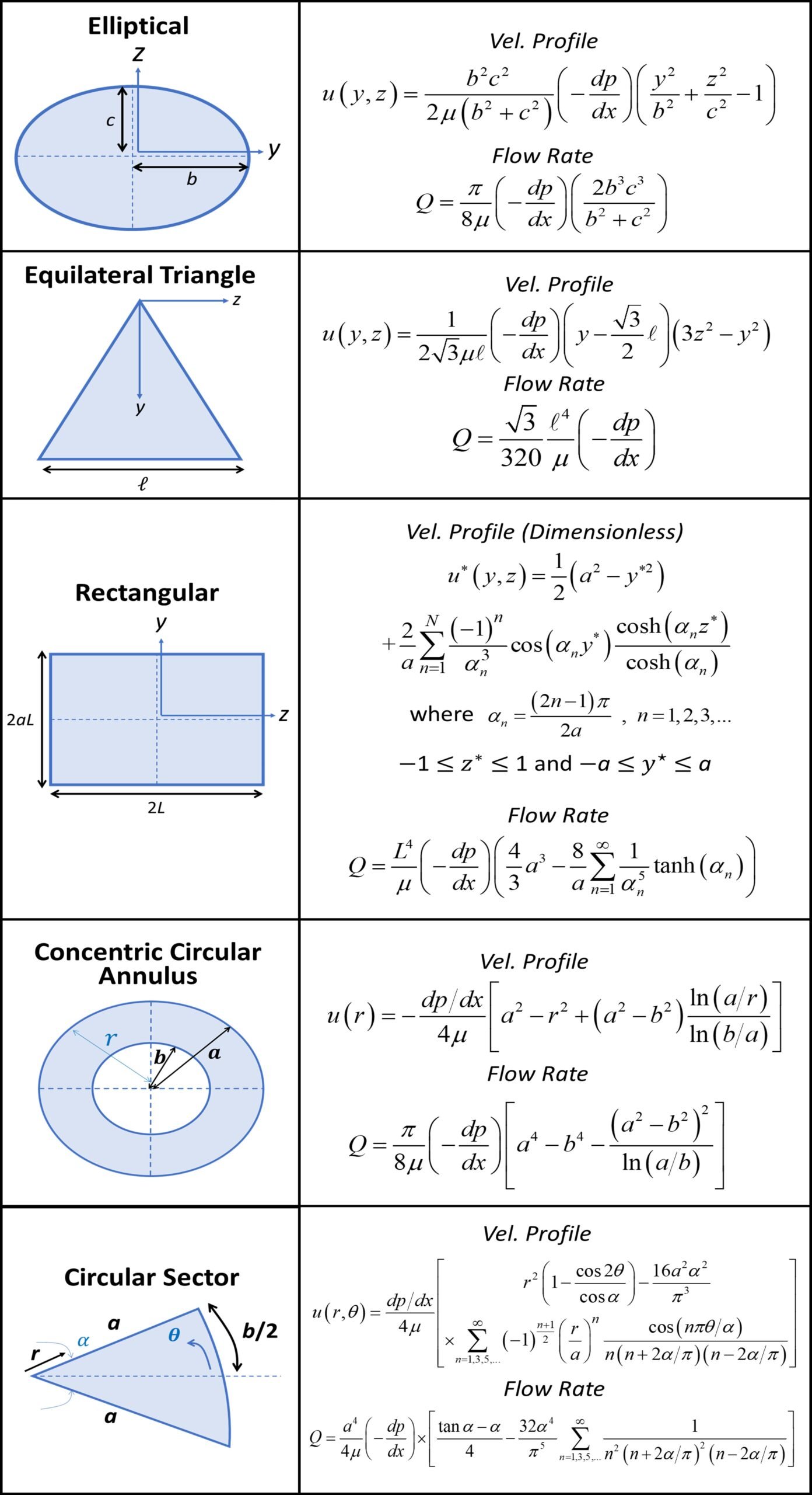
As indicated in Table 1, some types of section, such as the rectangle and the circular sector, are associated with rather intricate solutions. One way to avoid using these expressions while nonetheless achieving accurate results is to appeal to the concept of hydraulic diameter. The hydraulic diameter of a cross-section is the length measurement that represents a circular cross-section with proportions similar to those of the original geometry. It enables the modeler to use simple results and correlations that at first would not apply to, say, a rectangular or a circular-sector duct. Following White (2004), we define the hydraulic diameter as

where A and P are the area and wetted perimeter of the original cross-section, respectively. Since A has units of length squared and perimeter has units of length1, the ratio above likewise has units of length, hence the name ‘hydraulic diameter’. Once the hydraulic diameter of a section is established, a reasonable next step is to check whether the Reynolds number corresponding to Dh is within the range for laminar flow. The Reynolds number with hydraulic diameter as the reference length is of course
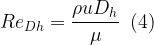
where 

Example 1 (White, 2004)
Air at 20oC and approximately 1 atm flows at an average velocity of 1.7 m/s through a rectangular 1 
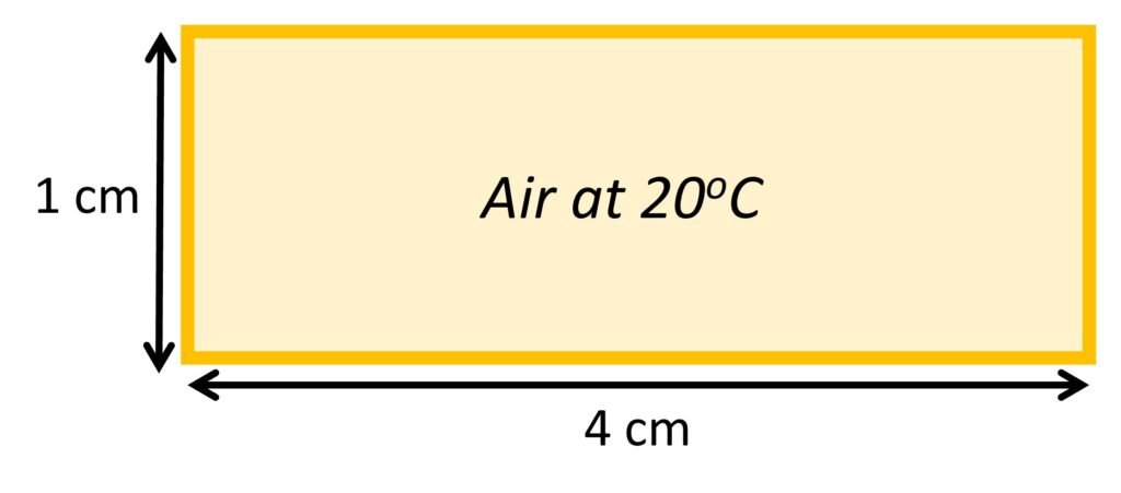
Solution. We first compute the hydraulic diameter:

![\displaystyle \therefore {{D}_{h}}=\frac{{4\times \left( {0.01\times 0.04} \right)}}{{\left[ {2\times \left( {0.01+0.04} \right)} \right]}}=0.016\,\text{m}](https://s0.wp.com/latex.php?latex=%5Cdisplaystyle+%5Ctherefore+%7B%7BD%7D_%7Bh%7D%7D%3D%5Cfrac%7B%7B4%5Ctimes+%5Cleft%28+%7B0.01%5Ctimes+0.04%7D+%5Cright%29%7D%7D%7B%7B%5Cleft%5B+%7B2%5Ctimes+%5Cleft%28+%7B0.01%2B0.04%7D+%5Cright%29%7D+%5Cright%5D%7D%7D%3D0.016%5C%2C%5Ctext%7Bm%7D&bg=ffffff&fg=000&s=1&c=20201002)
For air at 20oC and 1 atm, the density and dynamic viscosity are approximately 1.21 kg/m3 and 1.81
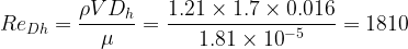
Since the Reynolds number is lower than 2000, we can surmise that flow is laminar. Now, beginning with the exact solution, the flow rate is given by
![\displaystyle Q=\frac{{{{L}^{4}}}}{\mu }\left( {-\frac{{dp}}{{dx}}} \right)\left[ {\frac{4}{3}{{a}^{3}}-\frac{8}{a}\sum\limits_{{n=1}}^{\infty }{{\frac{1}{{\alpha _{n}^{5}}}\tanh \left( {{{\alpha }_{n}}} \right)}}} \right]\,\,\,(\text{I})](https://s0.wp.com/latex.php?latex=%5Cdisplaystyle+Q%3D%5Cfrac%7B%7B%7B%7BL%7D%5E%7B4%7D%7D%7D%7D%7B%5Cmu+%7D%5Cleft%28+%7B-%5Cfrac%7B%7Bdp%7D%7D%7B%7Bdx%7D%7D%7D+%5Cright%29%5Cleft%5B+%7B%5Cfrac%7B4%7D%7B3%7D%7B%7Ba%7D%5E%7B3%7D%7D-%5Cfrac%7B8%7D%7Ba%7D%5Csum%5Climits_%7B%7Bn%3D1%7D%7D%5E%7B%5Cinfty+%7D%7B%7B%5Cfrac%7B1%7D%7B%7B%5Calpha+_%7Bn%7D%5E%7B5%7D%7D%7D%5Ctanh+%5Cleft%28+%7B%7B%7B%5Calpha+%7D_%7Bn%7D%7D%7D+%5Cright%29%7D%7D%7D+%5Cright%5D%5C%2C%5C%2C%5C%2C%28%5Ctext%7BI%7D%29&bg=ffffff&fg=000&s=1&c=20201002)
Its value is obtained by multiplying the velocity by the area of the cross-section:

The pressure drop dp/dx can be obtained by solving equation (I) for Q. Using Mathematica, let us compute the first few terms of the sum on the right-hand side:
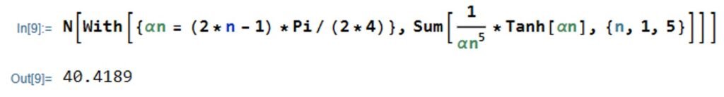
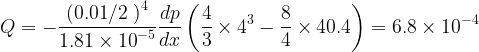
The sum is close to 40.4. Substituting in the expression for Q and solving for pressure gradient, we obtain


Now, to tackle this problem with the hydraulic diameter approach, we first note that the friction factor for laminar flow in a circular conduit is given by Cf = 16/Re, where Re is the Reynolds number:

Now, the average shear stress is given by the product of Cf and dynamic pressure:

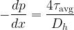
For fully developed flow, the relationship between pressure gradient and average wall shear is

The hydraulic diameter approach underestimates by approximately 10% the pressure drop obtained from the exact solution.
Example 2 (White, 2004)
It is desired to measure the viscosity of light lubricating oils (
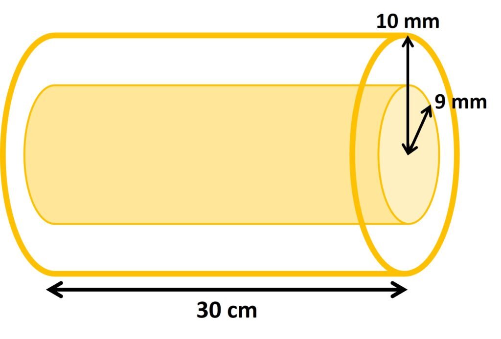
Solution. The area and perimeter of the annulus are, respectively:


The hydraulic diameter follows as

or approximately 2 mm. In turn, the average velocity is

Knowing that a typical oil has density of about 900 kg/m3, and that the oils measured have viscosities ranging from 0.02 Pa·s to 0.1 Pa·s, the Reynolds number will vary between

and

This interval of Re values is well within the laminar range, so we may use the solution in Table 1,
![\displaystyle Q=\frac{\pi }{{8\mu }}\frac{{dp}}{{dx}}\left[ {{{a}^{4}}-{{b}^{4}}-\frac{{{{{\left( {{{a}^{2}}-{{b}^{2}}} \right)}}^{2}}}}{{\ln \left( {{a}/{b}\;} \right)}}} \right]](https://s0.wp.com/latex.php?latex=%5Cdisplaystyle+Q%3D%5Cfrac%7B%5Cpi+%7D%7B%7B8%5Cmu+%7D%7D%5Cfrac%7B%7Bdp%7D%7D%7B%7Bdx%7D%7D%5Cleft%5B+%7B%7B%7Ba%7D%5E%7B4%7D%7D-%7B%7Bb%7D%5E%7B4%7D%7D-%5Cfrac%7B%7B%7B%7B%7B%5Cleft%28+%7B%7B%7Ba%7D%5E%7B2%7D%7D-%7B%7Bb%7D%5E%7B2%7D%7D%7D+%5Cright%29%7D%7D%5E%7B2%7D%7D%7D%7D%7B%7B%5Cln+%5Cleft%28+%7B%7Ba%7D%2F%7Bb%7D%5C%3B%7D+%5Cright%29%7D%7D%7D+%5Cright%5D&bg=ffffff&fg=000&s=1&c=20201002)
where Q = 1/3600 = 2.78

![\displaystyle Q=\frac{\pi }{{8\times 0.02}}\frac{{dp}}{{dx}}\left[ {{{{0.01}}^{4}}-{{{0.009}}^{4}}-\frac{{{{{\left( {{{{0.01}}^{2}}-{{{0.009}}^{2}}} \right)}}^{2}}}}{{\ln \left( {{{0.01}}/{{0.009}}\;} \right)}}} \right]=2.78\times {{10}^{{-4}}}](https://s0.wp.com/latex.php?latex=%5Cdisplaystyle+Q%3D%5Cfrac%7B%5Cpi+%7D%7B%7B8%5Ctimes+0.02%7D%7D%5Cfrac%7B%7Bdp%7D%7D%7B%7Bdx%7D%7D%5Cleft%5B+%7B%7B%7B%7B0.01%7D%7D%5E%7B4%7D%7D-%7B%7B%7B0.009%7D%7D%5E%7B4%7D%7D-%5Cfrac%7B%7B%7B%7B%7B%5Cleft%28+%7B%7B%7B%7B0.01%7D%7D%5E%7B2%7D%7D-%7B%7B%7B0.009%7D%7D%5E%7B2%7D%7D%7D+%5Cright%29%7D%7D%5E%7B2%7D%7D%7D%7D%7B%7B%5Cln+%5Cleft%28+%7B%7B%7B0.01%7D%7D%2F%7B%7B0.009%7D%7D%5C%3B%7D+%5Cright%29%7D%7D%7D+%5Cright%5D%3D2.78%5Ctimes+%7B%7B10%7D%5E%7B%7B-4%7D%7D%7D&bg=ffffff&fg=000&s=1&c=20201002)

or about 3.31 atm. Proceeding similarly with the most viscous oil (
![\displaystyle Q=\frac{\pi }{{8\times 0.1}}\frac{{dp}}{{dx}}\left[ {{{{0.01}}^{4}}-{{{0.009}}^{4}}-\frac{{{{{\left( {{{{0.01}}^{2}}-{{{0.009}}^{2}}} \right)}}^{2}}}}{{\ln \left( {{{0.01}}/{{0.009}}\;} \right)}}} \right]=2.78\times {{10}^{{-4}}}](https://s0.wp.com/latex.php?latex=%5Cdisplaystyle+Q%3D%5Cfrac%7B%5Cpi+%7D%7B%7B8%5Ctimes+0.1%7D%7D%5Cfrac%7B%7Bdp%7D%7D%7B%7Bdx%7D%7D%5Cleft%5B+%7B%7B%7B%7B0.01%7D%7D%5E%7B4%7D%7D-%7B%7B%7B0.009%7D%7D%5E%7B4%7D%7D-%5Cfrac%7B%7B%7B%7B%7B%5Cleft%28+%7B%7B%7B%7B0.01%7D%7D%5E%7B2%7D%7D-%7B%7B%7B0.009%7D%7D%5E%7B2%7D%7D%7D+%5Cright%29%7D%7D%5E%7B2%7D%7D%7D%7D%7B%7B%5Cln+%5Cleft%28+%7B%7B%7B0.01%7D%7D%2F%7B%7B0.009%7D%7D%5C%3B%7D+%5Cright%29%7D%7D%7D+%5Cright%5D%3D2.78%5Ctimes+%7B%7B10%7D%5E%7B%7B-4%7D%7D%7D&bg=ffffff&fg=000&s=1&c=20201002)


or about 16.5 atm. In summary, the device must be able to withstand pressure drops ranging from about 300 kPa to 1700 kPa. These are fairly high pressures, so a mechanical gage may be most appropriate.
3. Supremacy of the circular cross-section
To close this post, we propose a simple comparative treatment of circular cross-sections and their closest relatives – namely, elliptical sections. A generic elliptical cross-section is described by the equation

Taking b > c, the major and minor axes of the ellipse are respectively defined by

which means that the major and minor axes of the ellipse are 2b and 2c, respectively. As shown in Table 1, a solution for laminar, steady flow in an elliptical section is

where, for brevity, we have denoted the pressure gradient –dp/dx as k. To obtain the flow rate, we integrate the velocity profile (7) over the cross-section; specifically, the integration bounds are chosen for the first quadrant of the Cartesian plane, and the result is then multiplied by 4:
We may denote the rightmost factor as 

with the result that (8) can be restated as
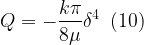
One quantity of interest is the so-called pumping power H, which can be obtained by multiplying the pressure gradient k = –dp/dx, the tube length L, and the flow rate Q; mathematically,

Solving (10) for k brings to

Since power is always positive, it makes sense to take the absolute value of the pressure gradient. Substituting in (11),

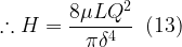
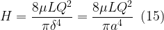
Equation (10) gives the flow rate for an elliptical duct, while (13) gives the power required to maintain such a flow. One noteworthy simplification arises if b = c = a, that is, when the two semiaxes b and c are both equal to some value a. In this case, we see that measurement becomes


That is,

which is simply the Poiseuille equation for flow in a circular duct (equation (2)). Similarly, substituting
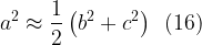
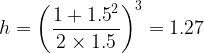
Zamir (2016) provides an interesting comparison between the relative efficiency of circular and elliptical cross-sections. In order to compare the performance of two cross-sections in conducting a fluid, we must first make equal either the perimeter or the area of the two sections. Zamir proposes the former approach, considering a circular cross-section of radius a and an elliptic cross-section of semiaxes b and c – that is, no different from our previous calculations. The perimeters of the two sections will be approximately equal if we have
Two scenarios arise in a comparative analysis of the two ducts: we can hold the pumping power fixed and allow the flow rate to vary; or we can hold the flow rate fixed and allow the pumping power to vary. In the first scenario, we have

For comparison, we denote as q the ratio of flow in an elliptic tube to flow in a circular tube. The value of q is

which, with Qellip and Qcirc taken from (10) and (14), respectively, becomes

Substituting

or, defining a ratio

In the second scenario, we make the flow rate fixed, so that
We denote as h the ratio of pumping power in an elliptic tube to pumping power in a circular tube. The value of h is

which, proceeding in a similar fashion as in (18), is found to be

Substituting Hellip and Hcirc from (13) and (15), respectively, and using the same ratio

The main findings of our comparative treatment stem from equations (19.2) and (22). Firstly, knowing that the ratio
As an example, suppose we have an elliptical cross-section for which the major semiaxis b is 1.5 times larger than the minor semiaxis c. In this case,

Thus, if the pumping power is to be the same in the elliptical tube and a circular tube with the same perimeter, the flow rate carried by the elliptical conduit will be about 21% less than the flow carried by the circular conduit. If, on the other hand, the flow rate were held fixed, ratio h in equation (22) would be
Thus, if the flow rate is to be the same in the elliptical tube and an equivalent circular tube, the elliptical conduit would require about 27% more pumping power than the circular conduit.
References
- PANTON, R.L. (2013). Incompressible Flow. 4th edition. Hoboken: John Wiley and Sons.
- WHITE, F.M. (2004). Viscous Fluid Flow. 3rd edition. New York: McGraw-Hill.
- ZAMIR, M. (2016). Hemo-Dynamics. Berlin/Heidelberg: Springer.

