Step-Growth Polymerization, the Carothers Equation, and the Flory-Schulz Distribution

In this article, we provide a brief quantitative treatment of step growth or condensation polymerization. We begin with an introduction to the Carothers equation; then, we proceed to a quick discussion on the Flory-Schulz molecular weight distribution; lastly, we provide a brief consideration of polymer gel points.

1. Deriving the Carothers equation (Rudin, 1982; Chanda, 2013; Reed and Alb, 2014)

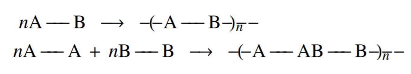
Calculations of the number-average degree of polymerization as a function of extent of reaction are very useful in designing and controlling step-growth polymerizations. The reactions we are considering may be summarized as in the figure below, where monomers carrying A-type functional groups react with B-type monomers. To be completely general, each functional group need not be confined to a single monomer, the functionalities of the various monomers may differ, and the functional groups of opposite kinds need not be present in equivalent quantities.

One crucial definition in the study of condensation polymerization is the concept of average functionality, defined by Rudin as

$\displaystyle {{f}_{{\text{av}}}}=\frac{{\Sigma {{N}_{i}}{{f}_{i}}}}{{\Sigma {{N}_{i}}}}$

where $\displaystyle {{N}_{i}}$ is the number of moles of species i with $\displaystyle {{f}_{i}}$ number of functional groups. The definition of average functionality presented above holds strictly when functional groups of opposite kinds are present in equal concentrations. If there is an excess of functional groups of one kind, the monomers carrying these groups will be able to react only until the opposite functional groups are consumed. In such nonstoichiometric mixtures the excess reactant does not enter the polymerization in the absence of side reactions and should not be counted in calculating $\displaystyle {{f}_{{av}}}$ . Consider a polymerization which forms AB links and in which $\displaystyle {{n}_{A}}$ > $\displaystyle {{n}_{B}}$ , where $\displaystyle {{n}_{i}}$ is the number of equivalents of functional groups of type i. In this case the number of B equivalents which can react cannot exceed $\displaystyle {{n}_{A}}$ , and therefore

$\displaystyle {{f}_{{av}}}=\frac{{2{{n}_{A}}}}{{\Sigma {{N}_{i}}}}=\frac{{2{{n}_{A}}}}{{{{N}_{A}}+{{N}_{B}}}}$

The initial number of monomers is $\displaystyle \Sigma {{N}_{i}}$ = $\displaystyle {{N}_{0}}$ , and $\displaystyle {{N}_{0}}{{f}_{{av}}}$ is the total number of useful equivalents of functional groups of all kinds that are present at the start of the reaction. We define p as the extent of reaction, equal to the fraction of functional groups in deficient concentration which have reacted. Obviously, 0 $\displaystyle \le$ p $\displaystyle \le$ 1, and p in stoichiometric mixtures is the fraction of functional groups of either kind or of both kinds which have reacted. Also, N is the total number of moles of molecules (monomer plus polymers of all sizes) when the reaction has proceeded to an extent p.

Neglecting intermolecular linkages, every time a new linkage is formed the reaction mixture will contain one less molecule. Therefore, when the number of molecules has been reduced from $\displaystyle {{N}_{0}}$ to $\displaystyle N$ moles the number of linkages which have been formed is equal to $\displaystyle {{N}_{0}}$ – $\displaystyle N$ moles. It takes two functional groups to form a linkage and so 2( $\displaystyle {{N}_{0}}$ – $\displaystyle N$ ) moles of functional groups will have been lost in forming these $\displaystyle {{N}_{0}}$ – $\displaystyle N$ moles of linkages. By definition,

$\displaystyle p=\frac{{\text{No}\text{. functional groups used}}}{{\text{No}\text{. functional groups initially}}}=\frac{{2\left( {{{N}_{0}}-N} \right)}}{{2{{N}_{0}}{{f}_{{av}}}}}$

Solving for $\displaystyle N$ , we have

$\displaystyle N=\frac{1}{2}\left( {2{{N}_{0}}-{{N}_{0}}p{{f}_{{\text{av}}}}} \right)$

The number average degree of polymerization of the reaction mixture is $\displaystyle {{\bar{X}}_{n}}$ , which is equal to the initial number of monomer units divided by the number of remaining molecules. In the present case,

$\displaystyle {{\bar{X}}_{n}}=\frac{{{{N}_{0}}}}{N}=\frac{{{{N}_{0}}}}{{\frac{1}{2}\left( {2{{N}_{0}}-{{N}_{0}}p{{f}_{{av}}}} \right)}}$

$\displaystyle \therefore {{\bar{X}}_{n}}=\frac{1}{{\frac{1}{2}\left( {2-p{{f}_{{\text{av}}}}} \right)}}$

$\displaystyle \therefore {{\bar{X}}_{n}}=\frac{2}{{2-p{{f}_{{\text{av}}}}}}\,\,\,(\text{I})$

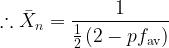
Equation (I) was proposed by Wallace Carothers of Dupont in the 1930s. Carothers was the inventor of nylon and the author of much of the polymer nomenclature used today. The quantitative dependence of $\displaystyle {{\bar{X}}_{n}}$ , and hence molecular weight, on the extent of reaction in condensation polymerization is made clear by the Carothers equation. From the corresponding data presented in the following table it is evident that to produce a relatively high-molecular-weight polymer ( $\displaystyle {{\bar{X}}_{n}}$ > 100), it is necessary to allow the reaction to proceed to a very high degree of conversion (p > 0.98), or, in other words, to a product that contains a very small number of chain ends. In general, this will be possible only when equal concentrations of the two reactive functional groups are maintained throughout the course of the reaction.

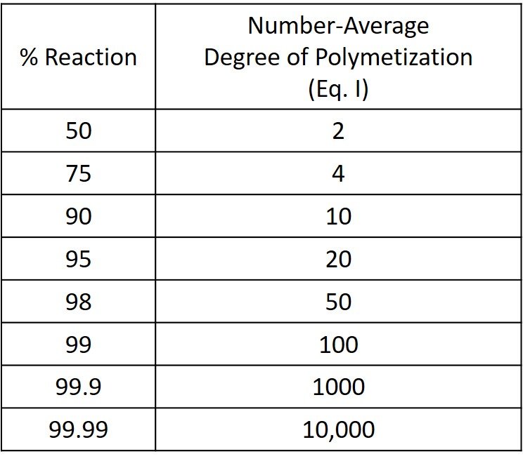
It is further evident from the previous table that $\displaystyle {{\bar{X}}_{n}}$ , and hence molecular weight, increases very rapidly with conversion in the high conversion range (p > 0.99). An increase in conversion from 0.99 to 0.999, for example, leads to a tenfold increase in $\displaystyle {{\bar{X}}_{n}}$ . It is thus not a realistic proposition to control polymer molecular weight by adjusting the extent of reaction. An alternative procedure to control $\displaystyle {{\bar{X}}_{n}}$ would be to introduce, deliberately, an imbalance in the ratio of the two types of functional groups in the feed. Another method of achieving the desired molecular weight is by addition of a small amount of a monofunctional monomer. The monofunctional monomer effectively caps the chain end it reacts with and prevents further growth of the chain. This is illustrated in Example 2.

Example 1 (Rudin, 1982)

Polybenzimidazoles are made by a two-stage step-growth melt polymerization:

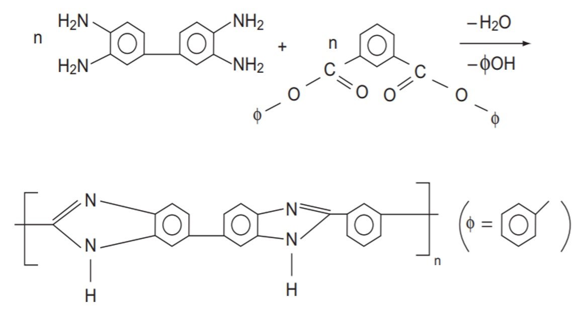
What extent of reaction is needed to produce n = 200?

Two NH₂ groups react with one COO $\displaystyle \phi$ group, so $\displaystyle f$ of each monomer is $\displaystyle {{f}_{{av}}}$ = 2. Since n = 200, it follows that $\displaystyle {{\bar{X}}_{n}}$ = 400. The extent of reaction follows from the Carothers equation,

$\displaystyle {{\bar{X}}_{n}}=\frac{2}{{2-p{{f}_{{av}}}}}=\frac{1}{{1-p}}$

so that, with $\displaystyle {{\bar{X}}_{n}}$ = 400,

$\displaystyle 400=\frac{1}{{1-p}}$

$\displaystyle \therefore p=0.9975\leftarrow$

A conversion of 99.75% is required to attain n = 200.

Example 2 (Modified from Rudin, 1982)

Poly(ethylenoxy benzoate), repeating unit MW = 164 g/mol, is a fiber-forming polymer produced by the following sequence of reactions:

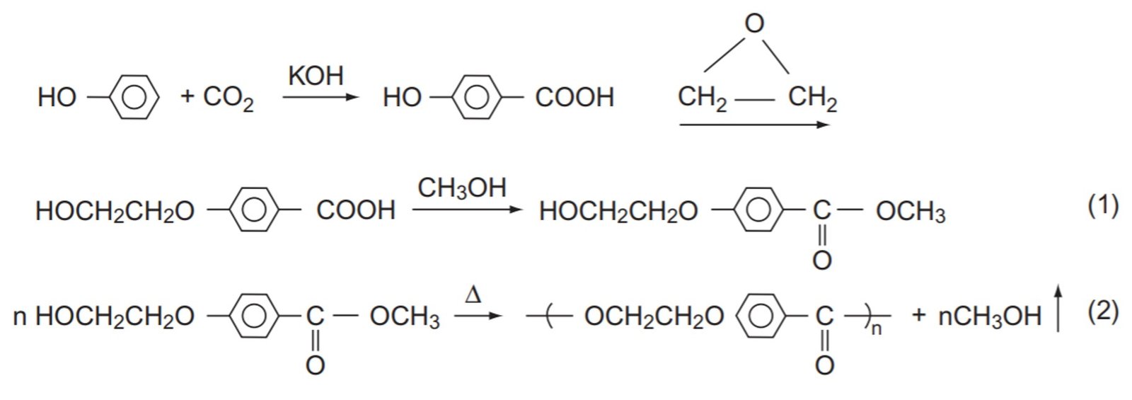
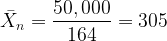
The polymer synthesis is a step-growth polymerization. The fiber is melt-spun at 250ºC – 270ºC and has silklike properties. It is known that the polymer becomes too viscous to spin conveniently when its number-average molecular weight exceeds 50,000. In order to prevent the product from exceeding this value, a small amount of methyl benzoate (structure illustrated below) is added to the mixture. How many moles of monofunctional ingredient per mole of monomer should be added to the mixture?

The number-average degree of polymerization should be no greater than

$\displaystyle {{\bar{X}}_{n}}=\frac{{50,000}}{{164}}=305$

From the Carothers equation with p $\displaystyle \to$ 1, we have

$\displaystyle {{\bar{X}}_{n}}=\frac{2}{{2-{{f}_{{\text{av}}}}}}=305$

$\displaystyle \therefore 2=305\left( {2-{{f}_{{av}}}} \right)$

$\displaystyle \therefore 305{{f}_{{\text{av}}}}=608$

$\displaystyle \therefore {{f}_{{\text{av}}}}=1.99344$

Let y be the number of moles of methyl benzoate in the mixture. The equivalents are computed in the following table.

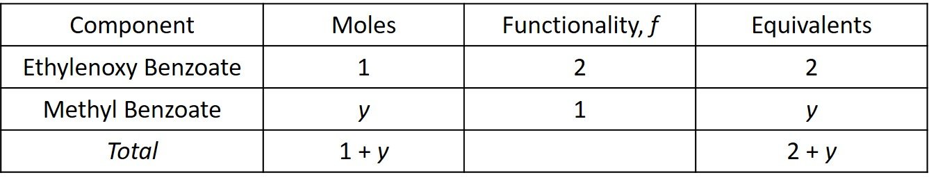
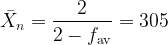
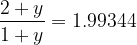
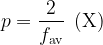
The average functionality $\displaystyle {{f}_{{av}}}$ is then

$\displaystyle {{f}_{{av}}}=\frac{{\Sigma \text{Equivalents}}}{{\Sigma \text{Moles}}}=\frac{{2+y}}{{1+y}}$

so that

$\displaystyle \frac{{2+y}}{{1+y}}=1.99344$

$\displaystyle \therefore 2+y=1.99344+1.99344y$

$\displaystyle \therefore 0.00656=0.99344y$

$\displaystyle \therefore y=\frac{{0.00656}}{{0.99344}}=0.00660\leftarrow$

Accordingly, 6.6 moles of monofunctional ingredient should be added for every kilomole of monomer.

2. Molecular weight distribution (Rudin, 1982; Chanda, 2013)

The molecular weight distribution (MWD) in ideal step growth polymerization was derived by Paul Flory in the 1950s and rediscovered by Günter Victor Schulz in the 1970s. Flory used the principle of equal reactivity of all functional groups of a given chemical type, irrespective of the size of the molecule to which they are attached; that is, the reactivity of each type of group does not change during the course of polymerization. The expression derived by Flory is

$\displaystyle {{w}_{x}}=x{{\left( {1-p} \right)}^{2}}{{p}^{{x-1}}}\,\,\,(\text{III})$

where $\displaystyle {{w}_{x}}$ is the weight fraction of x-mers (i.e., polymers consisting of x monomer residues) and p is the extent of reaction (which, in Flory’s statistical treatment, equates to the probability that a given group has reacted). Alternatively, the distribution equation can be restated in terms of the number (or moles) of molecules instead of a weight fraction. Let $\displaystyle {{n}_{x}}$ be the mole or number fraction of molecules in the polymer mixture that are x-mers. The probability that a given molecule is composed of exactly x units is

$\displaystyle {{n}_{x}}={{p}^{{x-1}}}\left( {1-p} \right)\,\,(\text{IV})$

In addition, $\displaystyle {{n}_{x}}$ is also given by

$\displaystyle {{n}_{x}}=\frac{{{{N}_{x}}}}{N}$

where $\displaystyle {{N}_{x}}$ is the number of molecules which are x-mers and $\displaystyle N$ is the total number of molecules at the extent of reaction p. With $\displaystyle {{N}_{x}}$ = $\displaystyle {{N}_{0}}$ (1 – p), in which $\displaystyle {{N}_{0}}$ is the initial number of molecules, the equation for $\displaystyle {{n}_{x}}$ can be restated as

$\displaystyle {{N}_{x}}={{N}_{0}}{{\left( {1-p} \right)}^{2}}{{p}^{{x-1}}}\,\,(\text{V})$

which is analogous to equation (III), the only difference being that the distribution is expressed in terms of number of molecules instead of mass.

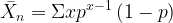
The Flory-Schulz model can be readily applied to derive expressions for the average degree of polymerization. The number-average degree of polymerization is given by

$\displaystyle {{\bar{X}}_{n}}=\frac{{\Sigma x{{N}_{x}}}}{{\Sigma {{N}_{x}}}}=\frac{{\Sigma x{{N}_{x}}}}{N}=\Sigma x{{n}_{x}}$

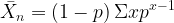
which, in view of equation (IV), becomes

$\displaystyle {{\bar{X}}_{n}}=\Sigma x{{p}^{{x-1}}}\left( {1-p} \right)$

Removing the (1 – p) term from the summation,

$\displaystyle {{\bar{X}}_{n}}=\left( {1-p} \right)\Sigma x{{p}^{{x-1}}}$

The summation on the right-hand side, with x ranging from zero to infinity, can be shown to yield

$\displaystyle \Sigma x{{p}^{{x-1}}}=\frac{1}{{{{{\left( {1-p} \right)}}^{2}}}}$

so that

$\displaystyle {{\bar{X}}_{n}}=\left( {1-p} \right)\times \frac{1}{{{{{\left( {1-p} \right)}}^{2}}}}=\frac{1}{{1-p}}\,\,\,(\text{VI})$

This expression has the same form as the Carothers equation, as one would expect. The weight-average degree of polymerization, in turn, is given by

$\displaystyle {{\bar{X}}_{w}}=\Sigma x{{w}_{x}}$

which, substituting $\displaystyle {{w}_{x}}$ from equation (III), becomes

$\displaystyle {{\bar{X}}_{w}}=\Sigma x\times \left[ {x{{{\left( {1-p} \right)}}^{2}}{{p}^{{x-1}}}} \right]=\Sigma {{x}^{2}}{{p}^{{x-1}}}{{\left( {1-p} \right)}^{2}}$

Removing the (1 – p)² term from the summation,

$\displaystyle {{\bar{X}}_{w}}={{\left( {1-p} \right)}^{2}}\Sigma {{x}^{2}}{{p}^{{x-1}}}$

The summation on the right-hand side, with x ranging from zero to infinity, can be shown to be

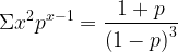
$\displaystyle \Sigma {{x}^{2}}{{p}^{{x-1}}}=\frac{{1+p}}{{{{{\left( {1-p} \right)}}^{3}}}}$

so that

$\displaystyle {{\bar{X}}_{w}}={{\left( {1-p} \right)}^{2}}\times \frac{{\left( {1+p} \right)}}{{{{{\left( {1-p} \right)}}^{3}}}}=\frac{{1+p}}{{1-p}}\,\,\,(\text{VII})$

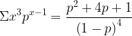
Lastly, the z-average degree of polymerization is given by the slightly more intricate formula

$\displaystyle {{\bar{X}}_{z}}=\frac{{\Sigma {{x}^{2}}{{w}_{x}}}}{{\Sigma x{{w}_{x}}}}$

Here,

$\displaystyle \Sigma {{x}^{2}}{{w}_{x}}=\Sigma {{x}^{3}}{{\left( {1-p} \right)}^{2}}{{p}^{{x-1}}}={{\left( {1-p} \right)}^{2}}\Sigma {{x}^{3}}{{p}^{{x-1}}}$

where the sum $\displaystyle \Sigma {{x}^{3}}{{p}^{{x-1}}}$ can be established with the Mathematica code

which returns

$\displaystyle \Sigma {{x}^{3}}{{p}^{{x-1}}}=\frac{{{{p}^{2}}+4p+1}}{{{{{\left( {1-p} \right)}}^{4}}}}$

so that

$\displaystyle \Sigma {{x}^{2}}{{w}_{x}}={{\left( {1-p} \right)}^{2}}\Sigma {{x}^{3}}{{p}^{{x-1}}}$

$\displaystyle \therefore \Sigma {{x}^{2}}{{w}_{x}}={{\left( {1-p} \right)}^{2}}\times \frac{{{{p}^{2}}+4p+1}}{{{{{\left( {1-p} \right)}}^{4}}}}=\frac{{{{p}^{2}}+4p+1}}{{{{{\left( {1-p} \right)}}^{2}}}}$

In addition, we know that

$\displaystyle \Sigma x{{w}_{x}}={{\bar{X}}_{w}}=\frac{{1+p}}{{1-p}}$

Combining the two previous results brings to

$\displaystyle {{\bar{X}}_{z}}=\frac{{\Sigma {{x}^{2}}{{w}_{x}}}}{{\Sigma x{{w}_{x}}}}=\frac{{\frac{{{{p}^{2}}+4p+1}}{{{{{\left( {1-p} \right)}}^{2}}}}}}{{\frac{{1+p}}{{1-p}}}}=\frac{{{{p}^{2}}+4p+1}}{{1-{{p}^{2}}}}\,\,\,(\text{VIII})$

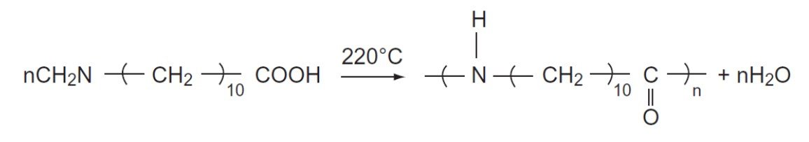
Example 3 (Modified from Rudin, 1982)

Nylon-11 is poly(11-aminoundecanoic acid), repeating unit molar mass 183 g/mol. This polymer has a critical melting point around 190ºC and has lower water absorption than nylon-6,6 or nylon-6. It can be used to make mechanical parts, packaging films, bristles, monofilaments, and sprayed and fluidized coatings.

A) How much monomer (in terms of weight fraction of the reaction mixture) is left when 90% of the functional groups have reacted?

B) At 90% conversion, calculate the weight fraction of the reaction mixture having a number-average degree of polymerization equal to 50.

C) At 90% conversion, compute the average molar masses $\displaystyle {{\bar{M}}_{n}}$ , $\displaystyle {{\bar{M}}_{w}}$ , and $\displaystyle {{\bar{M}}_{z}}$ .

A) The remaining weight fraction when 90% of the functional groups have reacted is given by the Flory-Schulz distribution with x = 1 and p = 0.9,

$\displaystyle {{w}_{x}}=x{{\left( {1-p} \right)}^{2}}{{p}^{{x-1}}}=1\times {{\left( {1-0.9} \right)}^{2}}\times {{0.9}^{{1-1}}}=0.01\leftarrow$

or 1 percent by weight.

B) From equation (III), with x = 50 and p = 0.9,

$\displaystyle {{w}_{{50}}}=50\times {{\left( {1-0.9} \right)}^{2}}\times {{0.9}^{{50-1}}}=0.00286\leftarrow$

or about 0.29 percent by weight.

C) The number-average degree of polymerization is given by equation (VI),

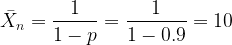
$\displaystyle {{\bar{X}}_{n}}=\frac{1}{{1-p}}=\frac{1}{{1-0.9}}=10$

so that

$\displaystyle {{\bar{M}}_{n}}=10\times 183=1830\leftarrow$

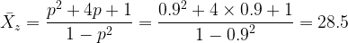
Next, the weight-average degree of polymerization is given by equation (VII),

$\displaystyle {{\bar{X}}_{w}}=\frac{{1+p}}{{1-p}}=\frac{{1+0.9}}{{1-0.9}}=19$

so that

$\displaystyle {{\bar{M}}_{w}}=19\times 183=3477\leftarrow$

Finally, the z-average degree of polymerization is given by equation (VIII),

$\displaystyle {{\bar{X}}_{z}}=\frac{{{{p}^{2}}+4p+1}}{{1-{{p}^{2}}}}=\frac{{{{{0.9}}^{2}}+4\times 0.9+1}}{{1-{{{0.9}}^{2}}}}=28.5$

so that

$\displaystyle {{\bar{M}}_{z}}=28.5\times 183=5220\leftarrow$

3. Polymer gelation

In the early stages of condensation polymerization, only linear and branched polymer molecules are present. However, as more and more crosslinks are formed, a point is reached when the reaction mixture forms essentially an infinite 3-D network. A sharp transition from a free-flowing viscous liquid to a gel may then occur and, for this reason, a polymer under such conditions is said to have reached the gel point. The gel point is defined as the state of conversion at which gel formation caused by crosslinking begins to become apparent. The Carothers equation can be used to estimate the conversion needed to reach the gel point in condensation polymerization involving monomers with functionalities higher than 2. With the assumption that the gel point is reached when practically all molecules of the limiting monomer have reacted, the requisite fractional conversion of functional groups can be estimated with a rearranged form of equation (II),

$\displaystyle p=\frac{2}{{{{f}_{{av}}}}}-\frac{2}{{{{{\bar{X}}}_{n}}{{f}_{{av}}}}}\,\,\,(\text{IX})$

This relationship is also, if somewhat redundantly, known as the Carothers equation. As the number-average degree of polymerization, $\displaystyle {{\bar{X}}_{n}}$ , is driven as high as possible, the second term on the right-hand side becomes negligible and the equation reduces to

$\displaystyle p=\frac{2}{{{{f}_{{\text{av}}}}}}\,\,\,(\text{X})$

For example, in condensation of an equimolar mixture of glycerol with a trifunctional acid such as citric acid, $\displaystyle {{f}_{{av}}}$ = 3 (both monomers are trifunctional), the gel point is reached at a functional conversion of groups of 2/3 = 0.667. It should be noted that gelation actually begins before all molecules of the limiting monomer have reacted, and the Carothers equation therefore tends to overestimate the conversion of functional groups needed to reach the gel point. Another limitation of this relation is that it may not predict the occurrence of gelation in systems that do present this phenomenon. For example, in the glycerol-phthalic anhydride polyesterification system, traces of diols and sometimes monocarboxylic acids are used to achieve relatively flexible products of lower cross-link density; gelation has been observed even when the mixture consists of equimolar proportions of glycerol, phthalic anhydride and a monofunctional acid, in spite of the fact that, for such mixtures, $\displaystyle {{f}_{{av}}}$ is exactly 2 and equation (X) predicts no such phenomenon at an extent of reaction lower than 1.

Example 4 (Rudin, 1982)

Consider the following alkyd recipe.

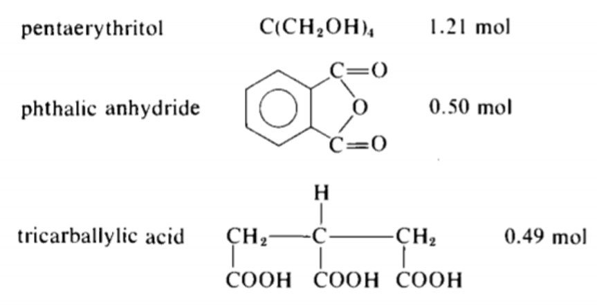
Can the above reaction be carried out to complete conversion without gelling?

The equivalents are computed in the following table.

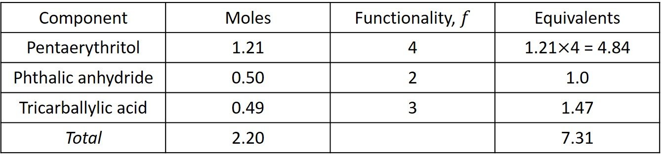
The total acid equivalents are 1.0 + 1.47 = 2.47 and the total OH equivalents are 4.84. Since the acid equivalents are in deficient supply, $\displaystyle {{f}_{{av}}}$ is determined with reference to the acid equivalents; that is,

$\displaystyle {{f}_{{\text{av}}}}=\frac{{2\times 2.47}}{{2.20}}=2.25$

Accordingly, the critical conversion is given by equation (X),

$\displaystyle {{p}_{c}}=\frac{2}{{{{f}_{{\text{av}}}}}}=\frac{2}{{2.25}}=0.889$

Since the acid groups are the limiting reactants, its conversion at the Carothers gel point is 0.889 < 1.0, which implies that complete conversion of COOH without gelation is not possible.

References

• CHANDA, M. (2013). Introduction to Polymer Science and Chemistry: A Problem-Solving Approach. 2nd edition. Boca Raton: CRC Press.

• REED, W. and ALB, A. (Eds.) (2014). Monitoring Polymerization Reactions: From Fundamentals to Applications. Hoboken: John Wiley and Sons.

• RUDIN, A. (1982). The Elements of Polymer Science and Engineering. Cambridge: Academic Press.

Step-Growth Polymerization, the Carothers Equation, and the Flory-Schulz Distribution

Subscribe to our Mailing List!

Featured Posts

A Primer on NAND Flash Memories

Solidification Time and Chvorinov’s Rule

More Articles

Aldohexoses: Classification, Haworth Projections, and Chair Conformations

Nuclear Binding Energy and the Semi-Empirical Mass Formula

Fields of Study

More

© 2024 Montogue Quiz

Subscribe to
our Mailing List!

Subscribe to our Mailing List!

Subscribe to receive our latest materials in your inbox.

Homework Help

© 2024 Montogue Quiz

Subscribe to our Mailing List!