In this blog post, I provide a quick introduction to the Grad-Shafranov equation, a seminal result in applied fusion physics that describes magnetohydrodynamic (MHD) equilibrium in torus-shaped reactors. In Section 1, I describe two preliminary concepts – a mathematical treatment of the theta-pinch and an introduction to the beta parameter – that will bolster the student’s understanding of the ensuing theory. In Section 2, the Grad-Shafranov equation is derived; the derivation is fairly complicated and requires some background on vector calculus and MHD, but even the unseasoned student will notice, especially from equation (42) onwards, that the theoretical underpinnings of the equation are actually simple. This becomes apparent in Section 3, where an elementary solution of the GS equation is used to derive the vertical magnetic field intensity required to sustain equilibrium in a tokamak. Finally, in Section 4 I present a full-fledged analytical solution to the GS equation and apply it to two real-life tokamaks. The last section is mainly drawn from Freidberg (2014), the closest source I found to Shafranov’s original solution in a 1966 paper published in a volume of Reviews of Plasma Physics. The advanced student is referred to Freidberg’s awesome textbook; Stacey (2005) and Morse (2018) are great, too.
1.Introduction: 
Our starting equation is the lowest-order momentum balance for a plasma under magnetohydrodynamic equilibrium:

That is, the pressure gradient equals the cross product of the current density and magnetic induction vectors. The current and the field must also satisfy Maxwell’s equations

and
The most immediate consequence of 


The vector product of

We see that there can be no perpendicular current in the absence of a pressure gradient.
The simplest confinement configuration to consider is radial equilibrium of cylindrical plasmas. We assume cylindrical symmetry so that all variables are independent of 

and the radial component of the momentum equation yields
![\displaystyle \frac{d}{{dr}}\left[ {P+\frac{{\left( {B_{\theta }^{2}+B_{z}^{2}} \right)}}{{2{{\mu }_{0}}}}} \right]=-\frac{{B_{\theta }^{2}}}{{{{\mu }_{0}}r}}\,\,\,(6)](https://s0.wp.com/latex.php?latex=%5Cdisplaystyle+%5Cfrac%7Bd%7D%7B%7Bdr%7D%7D%5Cleft%5B+%7BP%2B%5Cfrac%7B%7B%5Cleft%28+%7BB_%7B%5Ctheta+%7D%5E%7B2%7D%2BB_%7Bz%7D%5E%7B2%7D%7D+%5Cright%29%7D%7D%7B%7B2%7B%7B%5Cmu+%7D_%7B0%7D%7D%7D%7D%7D+%5Cright%5D%3D-%5Cfrac%7B%7BB_%7B%5Ctheta+%7D%5E%7B2%7D%7D%7D%7B%7B%7B%7B%5Cmu+%7D_%7B0%7D%7Dr%7D%7D%5C%2C%5C%2C%5C%2C%286%29&bg=ffffff&fg=000&s=1&c=20201002)
which expresses the (radial force) balance between the total (gas + magnetic) pressure gradient and the magnetic tension due to the curvature (if any) of the magnetic field. Of course, it is possible to remove magnetic curvature by choosing 
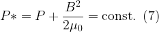
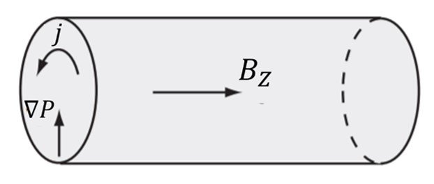
where P* is total pressure. Such a field can be produced by currents flowing azimuthally; early devices designed to contain plasma in this configuration were known as theta-pinches (since
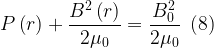
where 

i.e., the plasma is radially contained by the magnetic field generated by the azimuthal current flowing in its outer surface. If there is an internal magnetic field B(r), the current penetrates the plasma and (9) applies.
Figure 1. A
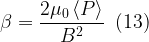
At this point, it is appropriate to introduce the normalized plasma pressure or beta parameter, a crucial figure of merit not only for the
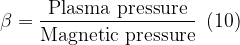
It is customary to define the plasma 


Accordingly, 


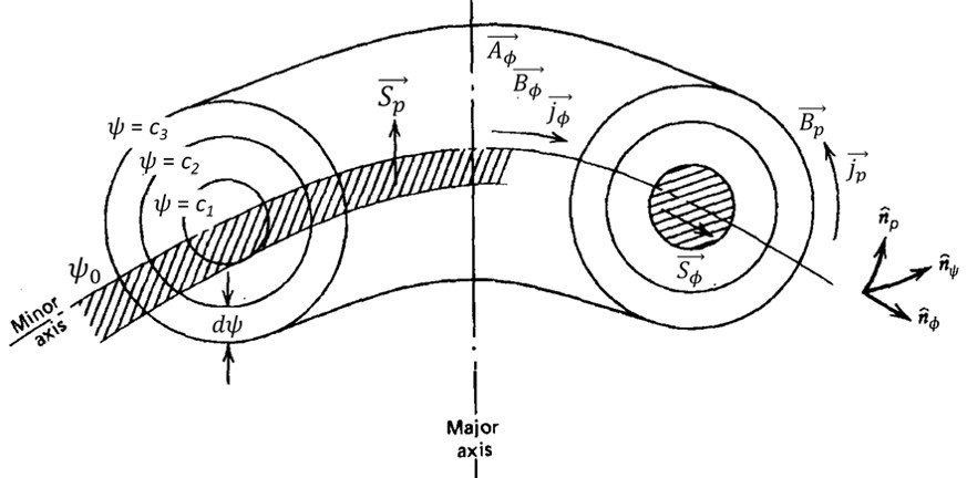
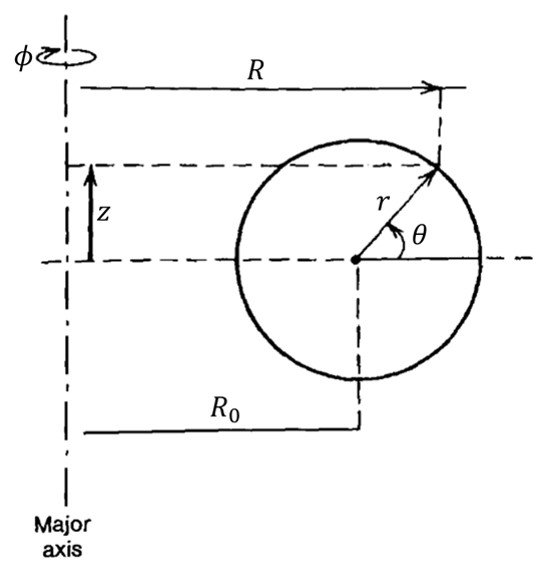
Figure 2. A reference torus cross-section.
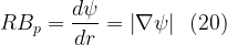
For the poloidal magnetic pressure a good choice for a circular cross-section plasma is 


where 
,
where 

It is often useful to define separate toroidal and poloidal
Importantly,

which indicates that the smaller of the two quantities 

2.The Grad-Shafranov equation (Stacey, 2005)
Devices such as the
The tokamak is the concept of interest in fusion research that has been shown to offer the best combination of toroidal and radial stability. Tokamaks have a large toroidal field and a small poloidal field with an aspect ratio on the order of R0/a 
In the following, we consider an axisymmetric, toroidal plasma with a toroidal plasma current. The isobaric surfaces are nested toroidal surfaces, not necessarily with circular cross-section (Figure 3). We define a function 


The magnetic axis is the innermost (degenerate) isobaric surface. Recalling that both the current and the field lie in the isobaric surfaces, it follows that the value of
Figure 3. Toroidal flux surfaces.
Now consider the incremental poloidal flux between adjacent flux surfaces (i.e., the poloidal flux passing through the planar ribbon extending from the isobaric surface labeled 


where R is the major radius from the major axis to the point in question. Accordingly, we see that
We are now able to construct a flux surface coordinate system (


and

The volume enclosed by the toroidal flux surface

and the differential volume of the toroidal annulus between

where 
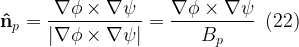
Using the results above, the magnetic field can be stated as

where

Because, by definition, 
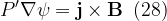
from which we immediately obtain

Using the requirement 

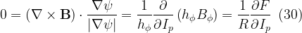
We know from axisymmetry that 


Using equation (26), the perpendicular current from (4) can be expressed in flux surface coordinates as
![\displaystyle {{\mathbf{j}}_{\bot }}=\frac{{{P}'}}{{{{B}^{2}}}}\left[ {F\left( {\nabla \phi \times \nabla \psi } \right)-{{{\left( {R{{B}_{p}}} \right)}}^{2}}\nabla \phi } \right]\,\,\,(31)](https://s0.wp.com/latex.php?latex=%5Cdisplaystyle+%7B%7B%5Cmathbf%7Bj%7D%7D_%7B%5Cbot+%7D%7D%3D%5Cfrac%7B%7B%7BP%7D%27%7D%7D%7B%7B%7B%7BB%7D%5E%7B2%7D%7D%7D%7D%5Cleft%5B+%7BF%5Cleft%28+%7B%5Cnabla+%5Cphi+%5Ctimes+%5Cnabla+%5Cpsi+%7D+%5Cright%29-%7B%7B%7B%5Cleft%28+%7BR%7B%7BB%7D_%7Bp%7D%7D%7D+%5Cright%29%7D%7D%5E%7B2%7D%7D%5Cnabla+%5Cphi+%7D+%5Cright%5D%5C%2C%5C%2C%5C%2C%2831%29&bg=ffffff&fg=000&s=1&c=20201002)
We conclude immediately that the perpendicular current lies in the flux surface, because 

lies in the flux surface, in agreement with our earlier observation. We now write

and use equations (31) and (32) to obtain

which indicates that the quantity in brackets is a constant on a flux surface, although it may vary with
![\displaystyle {{\mathbf{j}}_{{|\,|}}}=\left[ {-\frac{{{P}'F}}{B}\left( {1-\frac{{{{B}^{2}}}}{{\left\langle {{{B}^{2}}} \right\rangle }}} \right)+\frac{{B\left( {{{j}_{{|\,|}}}B} \right)}}{{\left\langle {{{B}^{2}}} \right\rangle }}} \right]{{\mathbf{\hat{n}}}_{{|\,|}}}\,\,\,(35)](https://s0.wp.com/latex.php?latex=%5Cdisplaystyle+%7B%7B%5Cmathbf%7Bj%7D%7D_%7B%7B%7C%5C%2C%7C%7D%7D%7D%3D%5Cleft%5B+%7B-%5Cfrac%7B%7B%7BP%7D%27F%7D%7D%7BB%7D%5Cleft%28+%7B1-%5Cfrac%7B%7B%7B%7BB%7D%5E%7B2%7D%7D%7D%7D%7B%7B%5Cleft%5Clangle+%7B%7B%7BB%7D%5E%7B2%7D%7D%7D+%5Cright%5Crangle+%7D%7D%7D+%5Cright%29%2B%5Cfrac%7B%7BB%5Cleft%28+%7B%7B%7Bj%7D_%7B%7B%7C%5C%2C%7C%7D%7D%7DB%7D+%5Cright%29%7D%7D%7B%7B%5Cleft%5Clangle+%7B%7B%7BB%7D%5E%7B2%7D%7D%7D+%5Cright%5Crangle+%7D%7D%7D+%5Cright%5D%7B%7B%5Cmathbf%7B%5Chat%7Bn%7D%7D%7D_%7B%7B%7C%5C%2C%7C%7D%7D%7D%5C%2C%5C%2C%5C%2C%2835%29&bg=ffffff&fg=000&s=1&c=20201002)
We have defined the flux surface average of a quantity A by
(We suppress the 
We can construct the toroidal and poloidal currents in the flux surface, (31) and (35),

and

These currents must be consistent with Ampère’s law. The toroidal and poloidal components of equation (2), in flux surface coordinates, are
and

Equating (38) and (40) results in the equation that must be satisfied by
Equating (37) and (39) and using (41) ultimately leads to

This general expression for axisymmetric, toroidal equilibria is known as the Grad-Shafranov equation. It is a nonlinear partial differential equation derived from the ideal MHD equations for static, toroidal equilibria with azimuthal symmetry (
Solutions to the Grad-Shafranov equation provide a complete characterization of axisymmetric ideal MHD equilibria. The nature of the equilibrium configuration is determined by the choice of the two arbitrary functions 

3.Asymptotic solutions and the vertical magnetic field (Stacey, 2005)
Although in practice solution of the Grad-Shafranov equation for magnetic flux surfaces is carried out numerically, it is useful to develop an approximate solution that provides significant physical insight. With this purpose in mind, we take the inverse aspect ratio

where R0 and a are the major and minor radii of the plasma, respectively. Conceptually, the plasma geometry in this case is more akin to a bicycle tire than a donut.
The solution of (42) for the flux surface function, 
![\displaystyle 2\pi \psi \left( {r,\theta } \right)=-{{\mu }_{0}}IR\left[ {\ln \left( {\frac{{8R}}{r}} \right)-2} \right]+\left\{ {-\frac{1}{2}{{\mu }_{0}}I\left[ {\ln \left( {\frac{{8R}}{r}} \right)-1} \right]r+\frac{{{{c}_{1}}}}{r}+{{c}_{2}}r} \right\}\cos \theta \,\,\,(43)](https://s0.wp.com/latex.php?latex=%5Cdisplaystyle+2%5Cpi+%5Cpsi+%5Cleft%28+%7Br%2C%5Ctheta+%7D+%5Cright%29%3D-%7B%7B%5Cmu+%7D_%7B0%7D%7DIR%5Cleft%5B+%7B%5Cln+%5Cleft%28+%7B%5Cfrac%7B%7B8R%7D%7D%7Br%7D%7D+%5Cright%29-2%7D+%5Cright%5D%2B%5Cleft%5C%7B+%7B-%5Cfrac%7B1%7D%7B2%7D%7B%7B%5Cmu+%7D_%7B0%7D%7DI%5Cleft%5B+%7B%5Cln+%5Cleft%28+%7B%5Cfrac%7B%7B8R%7D%7D%7Br%7D%7D+%5Cright%29-1%7D+%5Cright%5Dr%2B%5Cfrac%7B%7B%7B%7Bc%7D_%7B1%7D%7D%7D%7D%7Br%7D%2B%7B%7Bc%7D_%7B2%7D%7Dr%7D+%5Cright%5C%7D%5Ccos+%5Ctheta+%5C%2C%5C%2C%5C%2C%2843%29&bg=ffffff&fg=000&s=0&c=20201002)
with r 
![\displaystyle \Delta \left( r \right)=-\frac{{{{r}^{2}}}}{{2R}}\left[ {\ln \left( {\frac{{8R}}{r}} \right)-1} \right]+\frac{1}{{{{\mu }_{0}}IR}}\left( {{{c}_{1}}+{{c}_{2}}{{r}^{2}}} \right)\,\,\,(44)](https://s0.wp.com/latex.php?latex=%5Cdisplaystyle+%5CDelta+%5Cleft%28+r+%5Cright%29%3D-%5Cfrac%7B%7B%7B%7Br%7D%5E%7B2%7D%7D%7D%7D%7B%7B2R%7D%7D%5Cleft%5B+%7B%5Cln+%5Cleft%28+%7B%5Cfrac%7B%7B8R%7D%7D%7Br%7D%7D+%5Cright%29-1%7D+%5Cright%5D%2B%5Cfrac%7B1%7D%7B%7B%7B%7B%5Cmu+%7D_%7B0%7D%7DIR%7D%7D%5Cleft%28+%7B%7B%7Bc%7D_%7B1%7D%7D%2B%7B%7Bc%7D_%7B2%7D%7D%7B%7Br%7D%5E%7B2%7D%7D%7D+%5Cright%29%5C%2C%5C%2C%5C%2C%2844%29&bg=ffffff&fg=000&s=1&c=20201002)
Now, the magnetic field in the

Thus, the field outside the plasma is

![\displaystyle \therefore {{B}_{\theta }}=\frac{1}{{2\pi }}\left\{ {\frac{{{{\mu }_{0}}I}}{r}+\frac{1}{R}\left[ {-\frac{1}{2}{{\mu }_{0}}I\ln \left( {\frac{{8R}}{r}} \right)-\frac{{{{c}_{1}}}}{{{{r}^{2}}}}+{{c}_{2}}} \right]\cos \theta } \right\}\,\,\,(46)](https://s0.wp.com/latex.php?latex=%5Cdisplaystyle+%5Ctherefore+%7B%7BB%7D_%7B%5Ctheta+%7D%7D%3D%5Cfrac%7B1%7D%7B%7B2%5Cpi+%7D%7D%5Cleft%5C%7B+%7B%5Cfrac%7B%7B%7B%7B%5Cmu+%7D_%7B0%7D%7DI%7D%7D%7Br%7D%2B%5Cfrac%7B1%7D%7BR%7D%5Cleft%5B+%7B-%5Cfrac%7B1%7D%7B2%7D%7B%7B%5Cmu+%7D_%7B0%7D%7DI%5Cln+%5Cleft%28+%7B%5Cfrac%7B%7B8R%7D%7D%7Br%7D%7D+%5Cright%29-%5Cfrac%7B%7B%7B%7Bc%7D_%7B1%7D%7D%7D%7D%7B%7B%7B%7Br%7D%5E%7B2%7D%7D%7D%7D%2B%7B%7Bc%7D_%7B2%7D%7D%7D+%5Cright%5D%5Ccos+%5Ctheta+%7D+%5Cright%5C%7D%5C%2C%5C%2C%5C%2C%2846%29&bg=ffffff&fg=000&s=1&c=20201002)
and

![\displaystyle \therefore {{B}_{r}}=\frac{1}{{2\pi R}}\left\{ {-\frac{1}{2}{{\mu }_{0}}I\left[ {\ln \left( {\frac{{8R}}{r}} \right)-1} \right]+\frac{{{{c}_{1}}}}{{{{r}^{2}}}}+{{c}_{2}}} \right\}\sin \theta \,\,\,(47)](https://s0.wp.com/latex.php?latex=%5Cdisplaystyle+%5Ctherefore+%7B%7BB%7D_%7Br%7D%7D%3D%5Cfrac%7B1%7D%7B%7B2%5Cpi+R%7D%7D%5Cleft%5C%7B+%7B-%5Cfrac%7B1%7D%7B2%7D%7B%7B%5Cmu+%7D_%7B0%7D%7DI%5Cleft%5B+%7B%5Cln+%5Cleft%28+%7B%5Cfrac%7B%7B8R%7D%7D%7Br%7D%7D+%5Cright%29-1%7D+%5Cright%5D%2B%5Cfrac%7B%7B%7B%7Bc%7D_%7B1%7D%7D%7D%7D%7B%7B%7B%7Br%7D%5E%7B2%7D%7D%7D%7D%2B%7B%7Bc%7D_%7B2%7D%7D%7D+%5Cright%5C%7D%5Csin+%5Ctheta+%5C%2C%5C%2C%5C%2C%2847%29&bg=ffffff&fg=000&s=1&c=20201002)
This model can help us understand the confinement properties of toroidal plasmas. If the flux function is due entirely to the current flowing in the plasma – that is, there are no external fields – then the natural boundary condition 


![\displaystyle {{c}_{1}}=\frac{{{{\mu }_{0}}I}}{{2{{a}^{2}}}}\left[ {\ln \left( {\frac{{8R}}{a}} \right)-1} \right]\,\,\,(48)](https://s0.wp.com/latex.php?latex=%5Cdisplaystyle+%7B%7Bc%7D_%7B1%7D%7D%3D%5Cfrac%7B%7B%7B%7B%5Cmu+%7D_%7B0%7D%7DI%7D%7D%7B%7B2%7B%7Ba%7D%5E%7B2%7D%7D%7D%7D%5Cleft%5B+%7B%5Cln+%5Cleft%28+%7B%5Cfrac%7B%7B8R%7D%7D%7Ba%7D%7D+%5Cright%29-1%7D+%5Cright%5D%5C%2C%5C%2C%5C%2C%2848%29&bg=ffffff&fg=000&s=1&c=20201002)
In this case, equation (46) evaluated at the plasma surface is
![\displaystyle {{B}_{\theta }}\left( {a,\theta } \right)=\frac{{{{\mu }_{0}}I}}{{2\pi a}}\left\{ {1-\frac{a}{R}\left[ {\ln \left( {\frac{{8R}}{a}} \right)-\frac{1}{2}} \right]\cos \theta } \right\}\,\,\,(49)](https://s0.wp.com/latex.php?latex=%5Cdisplaystyle+%7B%7BB%7D_%7B%5Ctheta+%7D%7D%5Cleft%28+%7Ba%2C%5Ctheta+%7D+%5Cright%29%3D%5Cfrac%7B%7B%7B%7B%5Cmu+%7D_%7B0%7D%7DI%7D%7D%7B%7B2%5Cpi+a%7D%7D%5Cleft%5C%7B+%7B1-%5Cfrac%7Ba%7D%7BR%7D%5Cleft%5B+%7B%5Cln+%5Cleft%28+%7B%5Cfrac%7B%7B8R%7D%7D%7Ba%7D%7D+%5Cright%29-%5Cfrac%7B1%7D%7B2%7D%7D+%5Cright%5D%5Ccos+%5Ctheta+%7D+%5Cright%5C%7D%5C%2C%5C%2C%5C%2C%2849%29&bg=ffffff&fg=000&s=1&c=20201002)
If we now make the assumption that the plasma is a perfect conductor, we can arrive at some useful qualitative insights. Since there is no magnetic field within a perfect conductor, the magnetic pressure 


Figure 4. Magnetic fields affecting plasma equilibrium.
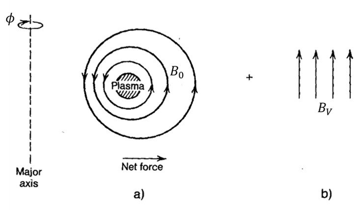
Now, we reformulate the solution under the assumption that the approximate solution to the GS equation given by (43) consists of a component due to the currents in the external coils or conducting shell and a component due to the plasma,
where

The constants c1 and c2 are now determined by requiring that the normal component of the field (

We likewise define a quantity 
Accordingly, the flux surface functions outside the plasma can be written
![\displaystyle 2\pi {{\psi }_{e}}=\frac{{{{\mu }_{0}}I}}{2}\left[ {\ln \left( {\frac{{8{{R}_{0}}}}{a}} \right)+\Lambda -\frac{1}{2}} \right]r\cos \theta \,\,\,(54)](https://s0.wp.com/latex.php?latex=%5Cdisplaystyle+2%5Cpi+%7B%7B%5Cpsi+%7D_%7Be%7D%7D%3D%5Cfrac%7B%7B%7B%7B%5Cmu+%7D_%7B0%7D%7DI%7D%7D%7B2%7D%5Cleft%5B+%7B%5Cln+%5Cleft%28+%7B%5Cfrac%7B%7B8%7B%7BR%7D_%7B0%7D%7D%7D%7D%7Ba%7D%7D+%5Cright%29%2B%5CLambda+-%5Cfrac%7B1%7D%7B2%7D%7D+%5Cright%5Dr%5Ccos+%5Ctheta+%5C%2C%5C%2C%5C%2C%2854%29&bg=ffffff&fg=000&s=1&c=20201002)
and
![\displaystyle 2\pi {{\psi }_{p}}=-{{\mu }_{0}}I{{R}_{0}}\left[ {\ln \left( {\frac{{8{{R}_{0}}}}{r}} \right)-2} \right]+\frac{1}{2}{{\mu }_{0}}I\left[ {-\ln \left( {\frac{{8{{R}_{0}}}}{r}} \right)+1-\frac{{{{a}^{2}}}}{{{{r}^{2}}}}\left( {\Lambda +\frac{1}{2}} \right)} \right]r\cos \theta \,\,\,(55)](https://s0.wp.com/latex.php?latex=%5Cdisplaystyle+2%5Cpi+%7B%7B%5Cpsi+%7D_%7Bp%7D%7D%3D-%7B%7B%5Cmu+%7D_%7B0%7D%7DI%7B%7BR%7D_%7B0%7D%7D%5Cleft%5B+%7B%5Cln+%5Cleft%28+%7B%5Cfrac%7B%7B8%7B%7BR%7D_%7B0%7D%7D%7D%7D%7Br%7D%7D+%5Cright%29-2%7D+%5Cright%5D%2B%5Cfrac%7B1%7D%7B2%7D%7B%7B%5Cmu+%7D_%7B0%7D%7DI%5Cleft%5B+%7B-%5Cln+%5Cleft%28+%7B%5Cfrac%7B%7B8%7B%7BR%7D_%7B0%7D%7D%7D%7D%7Br%7D%7D+%5Cright%29%2B1-%5Cfrac%7B%7B%7B%7Ba%7D%5E%7B2%7D%7D%7D%7D%7B%7B%7B%7Br%7D%5E%7B2%7D%7D%7D%7D%5Cleft%28+%7B%5CLambda+%2B%5Cfrac%7B1%7D%7B2%7D%7D+%5Cright%29%7D+%5Cright%5Dr%5Ccos+%5Ctheta+%5C%2C%5C%2C%5C%2C%2855%29&bg=ffffff&fg=000&s=0&c=20201002)
The components of the field due to the external coils in an (

![\displaystyle {{B}_{{V,R}}}=\frac{1}{R}\frac{{\partial {{\psi }_{e}}}}{{\partial z}}=-\frac{{{{\mu }_{0}}I}}{{4\pi R}}\left[ {\ln \left( {\frac{{8{{R}_{0}}}}{a}} \right)+\Lambda -\frac{1}{2}} \right]\tan \theta \,\,\,\left( {r>a} \right)\,\,\,(56)](https://s0.wp.com/latex.php?latex=%5Cdisplaystyle+%7B%7BB%7D_%7B%7BV%2CR%7D%7D%7D%3D%5Cfrac%7B1%7D%7BR%7D%5Cfrac%7B%7B%5Cpartial+%7B%7B%5Cpsi+%7D_%7Be%7D%7D%7D%7D%7B%7B%5Cpartial+z%7D%7D%3D-%5Cfrac%7B%7B%7B%7B%5Cmu+%7D_%7B0%7D%7DI%7D%7D%7B%7B4%5Cpi+R%7D%7D%5Cleft%5B+%7B%5Cln+%5Cleft%28+%7B%5Cfrac%7B%7B8%7B%7BR%7D_%7B0%7D%7D%7D%7D%7Ba%7D%7D+%5Cright%29%2B%5CLambda+-%5Cfrac%7B1%7D%7B2%7D%7D+%5Cright%5D%5Ctan+%5Ctheta+%5C%2C%5C%2C%5C%2C%5Cleft%28+%7Br%3Ea%7D+%5Cright%29%5C%2C%5C%2C%5C%2C%2856%29&bg=ffffff&fg=000&s=1&c=20201002)
and
![\displaystyle {{B}_{{V,Z}}}=\frac{1}{R}\frac{{\partial {{\psi }_{e}}}}{{\partial R}}=\frac{{{{\mu }_{0}}I}}{{4\pi R}}\left[ {\ln \left( {\frac{{8{{R}_{0}}}}{a}} \right)+\Lambda -\frac{1}{2}} \right]\,\,\,\left( {r>a} \right)\,\,\,(57)](https://s0.wp.com/latex.php?latex=%5Cdisplaystyle+%7B%7BB%7D_%7B%7BV%2CZ%7D%7D%7D%3D%5Cfrac%7B1%7D%7BR%7D%5Cfrac%7B%7B%5Cpartial+%7B%7B%5Cpsi+%7D_%7Be%7D%7D%7D%7D%7B%7B%5Cpartial+R%7D%7D%3D%5Cfrac%7B%7B%7B%7B%5Cmu+%7D_%7B0%7D%7DI%7D%7D%7B%7B4%5Cpi+R%7D%7D%5Cleft%5B+%7B%5Cln+%5Cleft%28+%7B%5Cfrac%7B%7B8%7B%7BR%7D_%7B0%7D%7D%7D%7D%7Ba%7D%7D+%5Cright%29%2B%5CLambda+-%5Cfrac%7B1%7D%7B2%7D%7D+%5Cright%5D%5C%2C%5C%2C%5C%2C%5Cleft%28+%7Br%3Ea%7D+%5Cright%29%5C%2C%5C%2C%5C%2C%2857%29&bg=ffffff&fg=000&s=1&c=20201002)
where we have made use of the relationships (see Figure 5)


Formulas (56) and (57) provide valuable information about the design requirements for the vertical field circuit, in particular how large the vertical field must be to center the plasma as a function of toroidal current and geometry.
Figure 5. Relation of (
4.Analytic solution (Freidberg, 2014)
As shown in the previous section, use of asymptotic expansions in small 
Following Freidberg (2014), we denote the free functions F and P in such a manner that
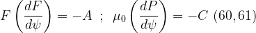
where A and C are constants. The surfaces defined by (60) and (61) are known as Solov’ev profiles. With these choices the Grad-Shafranov equation becomes

At this point it is useful to normalize the flux function and the coordinates as follows: 


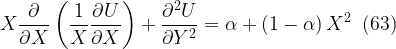
Here, 
There is now a crucial difference in the way that the exact equation is solved as compared to the asymptotic approach. In the latter, a standard approach is used. A surface is specified, for instance a circle or ellipse, and the equations are solved subject to the boundary conditions of regularity and
This approach does not really work for the exact problem because simple analytic solutions cannot be found that exactly satisfy the boundary conditions on simple surfaces such as a circle or an ellipse. Instead, the approach used is to find an exact analytic solution to equation (62) consisting of the superposition of a finite number of terms each with an undetermined multiplicative amplitude. A series of boundary constraints is then applied, forcing the analytic solutions to match a finite number of specified conditions on a known desired surface – one boundary constraint for each unknown multiplicative amplitude. The resulting solution is then uniquely defined. One then simply plots the contours of U = constant, including the plasma surface U = 0. Obviously, matching properties at a finite number of points does not guarantee that the resulting U = 0 surface will be close to the desired matching surface at all points. One must just take whatever the solution produces. The mathematical challenges to make this approach work involve choosing (1) the right set of analytic basis functions, (2) the right number of terms in the finite sum, and (3) the right set of matching constraints, so that the resulting U = 0 surface closely matches the desired surface for a very wide range of plasma parameters.
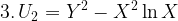
The solution to (62) consists of particular and homogeneous contributions. A convenient way to write the particular solution is the following:

The homogeneous solution, in turn, satisfies

Simple basis functions that exactly satisfy (62) consist of combinations of polynomials in X and Y. The exact form of each polynomial solution can be easily found by direct substitution. The approach used here assumes that the overall solution can be written as a Taylor series in these polynomial solutions, starting from a constant and increasing up to and including sixth-order terms. Truncating the series at sixth-order polynomials is not an obvious choice and indeed was arrived at by trial and error. At any rate, the exact analytic solution to the Grad-Shafranov equation used to model tokamaks is given by


Observe that all the polynomials are even in Y, indicating that attention is focused on up-down symmetric configurations.
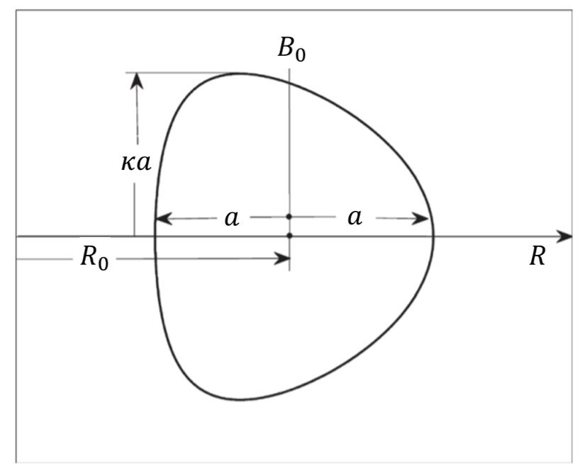
The task now is to define seven boundary constraints that will serve to determine the seven unknown coefficients cj. These constraints are chosen to match seven properties on a known desired plasma surface. A good choice for this reference surface, which is often used in the fusion community, is given parametrically in terms of variable 


The surface and corresponding geometry are illustrated in Figure 6. As can be seen, eqs. (67) and (68) parametrize a “D” shaped contour in terms of three dimensionless parameters: the inverse aspect ratio 


Here, Nj are curvature coefficients that can be determined from the model surface,


Once the free constants A and C or, equivalently,
The last step in the formulation is to derive relationships for the figures of merit q* (the kink safety factor),


![\displaystyle {{\beta }_{t}}=\left[ {\frac{{8{{\pi }^{2}}{{\varepsilon }^{4}}\left( {1-\alpha } \right)}}{{q_{*}^{2}}}} \right]{{\left( {\frac{{1+{{\kappa }^{2}}}}{2}} \right)}^{2}}\frac{{{{K}_{2}}}}{{K_{1}^{2}{{K}_{3}}}}\,\,\,(74)](https://s0.wp.com/latex.php?latex=%5Cdisplaystyle+%7B%7B%5Cbeta+%7D_%7Bt%7D%7D%3D%5Cleft%5B+%7B%5Cfrac%7B%7B8%7B%7B%5Cpi+%7D%5E%7B2%7D%7D%7B%7B%5Cvarepsilon+%7D%5E%7B4%7D%7D%5Cleft%28+%7B1-%5Calpha+%7D+%5Cright%29%7D%7D%7B%7Bq_%7B%2A%7D%5E%7B2%7D%7D%7D%7D+%5Cright%5D%7B%7B%5Cleft%28+%7B%5Cfrac%7B%7B1%2B%7B%7B%5Ckappa+%7D%5E%7B2%7D%7D%7D%7D%7B2%7D%7D+%5Cright%29%7D%5E%7B2%7D%7D%5Cfrac%7B%7B%7B%7BK%7D_%7B2%7D%7D%7D%7D%7B%7BK_%7B1%7D%5E%7B2%7D%7B%7BK%7D_%7B3%7D%7D%7D%7D%5C%2C%5C%2C%5C%2C%2874%29&bg=ffffff&fg=000&s=1&c=20201002)
where
![\displaystyle {{K}_{1}}=\int{{dXdY\left[ {\frac{{\alpha +\left( {1-\alpha } \right){{X}^{2}}}}{X}} \right]}}\,\,\,(75)](https://s0.wp.com/latex.php?latex=%5Cdisplaystyle+%7B%7BK%7D_%7B1%7D%7D%3D%5Cint%7B%7BdXdY%5Cleft%5B+%7B%5Cfrac%7B%7B%5Calpha+%2B%5Cleft%28+%7B1-%5Calpha+%7D+%5Cright%29%7B%7BX%7D%5E%7B2%7D%7D%7D%7D%7BX%7D%7D+%5Cright%5D%7D%7D%5C%2C%5C%2C%5C%2C%2875%29&bg=ffffff&fg=000&s=1&c=20201002)


Figure 6. Geometry of the reference surface.
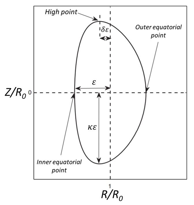
Table 1 summarizes characteristics of the TFTR and JET tokamaks.
Table 1. Characteristics of the TFTR and JET tokamaks.
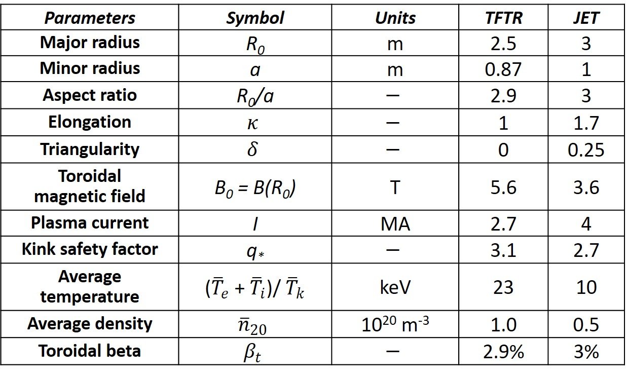
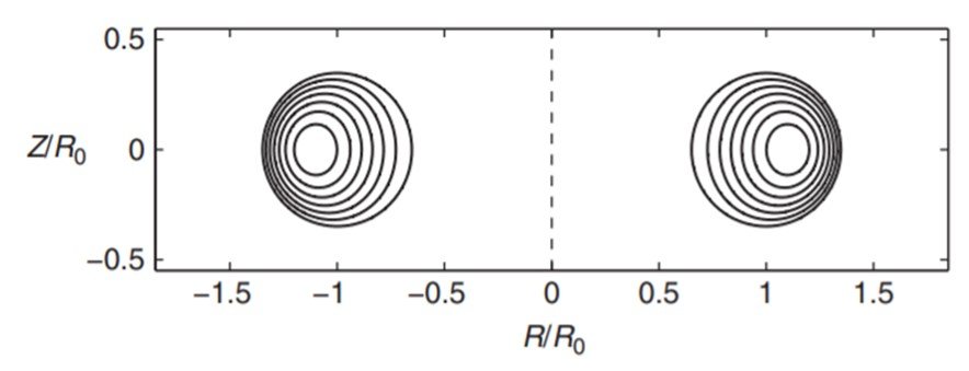
The simplest initial test of the analytic solution procedure is Princeton’s Tokamak Fusion Test Reactor (TFTR), which has a circular cross-section and MHD parameters summarized in Table 1. The analytic solution procedure is applied and the resulting flux surfaces are illustrated in Figure 7. As can be seen, the solution reliably reproduces shifted circular flux surface equilibria.
Figure 7. Exact Solov’ev equilibrium for TFTR.
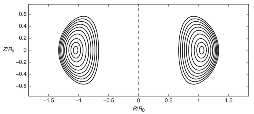
Another device that can be modelled by the analytical procedure outlined above is the Joint European Torus (JET). Although JET normally operates with a divertor, the analytic procedure assumes that the surface has been smoothed out. JET in fact is a relatively easy test for the equilibrium procedure. Using the values given above, the equilibrium flux surfaces for the solution profiles have been calculated and are illustrated in Figure 8. Observe the elongated “D” shaped plasma and the finite shift of the magnetic axis. The flux surfaces are smooth and nested, showing that the analytic solutions provide a credible representation of high-performance JET equilibria.
Figure 8. Exact Solov’ev equilibrium for JET.
References
• BOYD, T.J.M. and SANDERSON, J.J. (2003). The Physics of Plasmas. Cambridge: Cambridge University Press.
• FREIDBERG, J.P. (2014). Ideal MHD. Cambridge: Cambridge University Press.
• MORSE, E. (2018). Nuclear Fusion. Berlin/Heidelberg: Springer.
• Shafranov, V.D. (1966). Plasma equilibrium in a magnetic field. In: LEONTOVICH, M.A. (Ed.). Reviews of Plasma Physics, Vol. 2. New York: Consultants Bureau.
• STACEY, W.M. (2005). Fusion Plasma Physics. Weinheim: Wiley-VCH.
• WESSON, J. (2004). Tokamaks. Oxford: Clarendon Press.