

1. The basic Hoek-Brown failure criterion
The Hoek-Brown failure criterion is a nonlinear, empirical approach to the mechanical behavior of rock under conditions close to, or precisely at, mechanical failure. The criterion derives from Hoek’s (1968) studies with brittle rock failure, which in turn were loosely based on the crack theory developed by Griffith in the 1920s. The model was introduced in 1980 by Evert Hoek, arguably the most accomplished rock mechanicist of the past 50 years, and his regular collaborator Edwin T. Brown of the University of Queensland; it has since become a well-established tool for engineers dealing with rock slopes, rock foundations, tunneling, and other situations of civil and mining interest.
In developing their model, Hoek and Brown (1980) analyzed conventional triaxial test data for more than 14 intact rock types covering a number of igneous, sedimentary and metamorphic rocks with peak strengths ranging from 40 MPa for a sandstone to 580 MPa for a chert. The analysis included multiple tests for the same rock type carried out in different laboratories and only considered datasets containing a minimum of five tests covering a range of confining stresses. The coefficient of determination for most stress data ranged from 0.68 to 0.99, with most being greater than 0.9.
The original derivation of the Hoek-Brown criterion assumes that rock failure is controlled only by the major and minor principal stresses, 


The original form of the Hoek-Brown failure criterion can be stated as
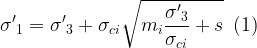
where 


As can be seen, the relationship between the effective principal stresses at failure for a given rock is defined by two constants, namely the uniaxial compressive strength
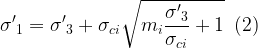
Figure 1. A Hoek-Brown failure envelope.
When the Hoek-Brown failure criterion was introduced, it was recommended that triaxial test results should be analyzed by linear regression of the following version of equation (2),

This approach was used for several years until it was realized that the method was inadequate for the analysis of data other than closely spaced points with very little scatter about a trend line (Hoek, 2018). A variety of methods are available for fitting curves through non-uniform distributions of triaxial test data. One of these, known as the modified Cuckoo search (Walton et al., 2011), is included in the Rocscience program RocData, which can be used for the interpretation of laboratory test data.
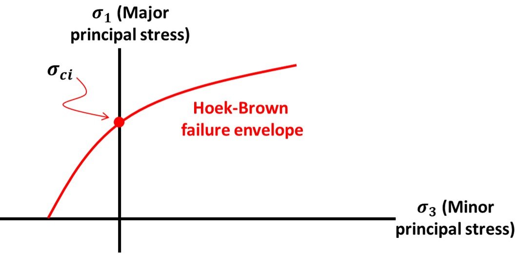
In an analogy with the Mohr-Coulomb failure criterion, the mi and s parameters are somewhat equivalent to the friction angle 
Figure 2. A Hoek-Brown failure envelopes for various values of mi
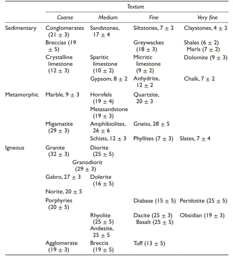
Although little significance was attributed to the mi parameter in the first few decades of collective experience with the Hoek-Brown criterion, research by Zuo et al. (2008, 2015) showed that mi in fact has physical meaning in a micromechanics context. It has been shown that mi can be written as

where 


Table 1. Typical values of the Hoek-Brown constant mi. Values in parentheses are estimates. Others are measured.
2. The tension cutoff
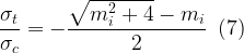
The intercept of the Hoek-Brown parabola with the 

which is a second-degree equation with solution

The right-hand side depends on the two constants of the model and can be readily determined; things get even easier for intact rock, in which case s = 1 and
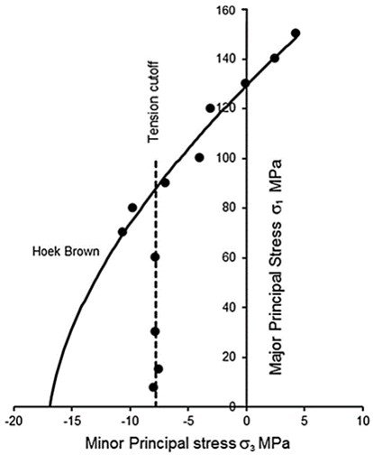
The result above indicates that knowledge of the mi constant and the uniaxial compressive strength suffices to estimate the tensile strength of a rock mass, or, equivalently, that the horizontal intercept of the Hoek-Brown failure envelope can serve as a decent estimate of tensile strength. However, this approach is vehemently contested in Hoek and Martin (2014). In that paper, Hoek and his collaborator refer to studies in which the tensile behavior of rocks had been investigated in the context of failure criteria. The results of one particular set of tests, drawn from the work of Ramsey and Chester (2004) on Carrara marble, are reproduced in Figure 3. The Hoek-Brown criterion was fitted to the shear data obtained in these tests and the resulting curve has been projected back to give an intercept of
Figure 3. Results from confined extension tests and triaxial compression tests by Ramsey and Chester (2004).
It has been shown that the tensile failure behavior of rock can be better represented by a modified version of Griffith failure criterion as proposed by Fairhurst (1964). This criterion is fundamentally based on the ratio of compressive to tensile strength, 
Figure 4. Dimensionless plot of triaxial test results from laboratory tests on samples from a wide range of rock types and concrete.

3. The generalized Hoek-Brown failure criterion
The generalized Hoek-Brown criterion for the estimation of rock mass strength, introduced by Hoek (1994) and Hoek et al. (1995), is expressed as

The rock mass scaling relationships for mb, s and a were reported as

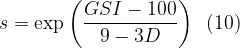

In these expressions, mi is the Hoek-Brown constant for intact rock, GSI is the geological strength index for the rock mass under consideration, and D is the blast damage factor. The uniaxial compressive strength of the rock mass,

The tensile strength of the rock mass, with all the reservations posed in the previous section, is obtained by setting

Note that 
The exponential term a in the generalized Hoek-Brown failure criterion was introduced to address the system’s bias towards hard rock and to better account for poorer-quality rock masses by enabling the curvature of the failure envelope to be adjusted, particularly under very low normal stresses. Inspection of equations (9) to (11) shows that in order to use the generalized Hoek-Brown criterion in the description of strength and deformability of jointed rock masses, four ‘properties’ of the rock mass have to be known beforehand. These are
- The uniaxial compressive strength
- The value of the Hoek-Brown constant mi for the intact rock pieces.
- The Geological Strength Index (GSI) for the rock mass.
- The blast damage factor D.
The uniaxial compressive strength
3.1. The Geological Strength Index (GSI)
The Geological Strength Index was introduced by Hoek (1994) and further developed in a number of papers published over the course of the 1990s. Hoek noticed that a failure criterion such as the one that he had published with Brown in the previous decade would be useless in practical work if it could not be easily linked to field observations of a rock mass. At that time, rock classification schemes such as Bieniawski’s Rock Mass Rating (RMR) and Barton’s Q-system were available, but mechanical modelling of rock masses was not an overarching application in either of them. Thus, Hoek introduced a new classification system, the Geological Strength Index, with rock mechanical strength and deformation in mind. Hoek proposed a very simple relation between the GSI score and Bieniawski’s RMR,

where RMR89 denotes the rock mass rating in the 1989 version of the RMR (Bieniawski, 1989). This simple relation ensured that adherents to the well-seasoned Rock Mass Rating system could easily switch to Hoek’s new approach. The transition between systems was quite straightforward because, unlike the RMR, which relies on a summation of numerical contributions related to different aspects of the rock mass, the GSI score could be obtained simply by mapping visual observations of two aspects of the rock mass – rock structure and surface discontinuity conditions – onto a single standard chart. As a result, rock mechanicists gradually stopped using equation (14) to convert their RMR scores to the new system, and instead began employing the GSI chart and its associated methodology directly. Another reason for scrapping the RMR in correlations for use with the HB criterion was that the RMR was better tailored for rock masses of good quality, i.e. those with rating greater than 30 or so, but was difficult to apply to rocks of very poor quality (Zuo and Shen, 2020). Based on experience with difficult rock mass materials encountered in tunneling projects in Greece, Hoek et al. (1998) and Marinos and Hoek (2001) proposed a general GSI system that includes poor-quality rock masses. The GSI chart in its current iteration is reproduced in Figure 5. A simple description of rock mass quality on the basis of GSI is provided in Table 2.
Figure 5. Geological Strength Index (GSI) chart. After Marinos and Hoek (2001).
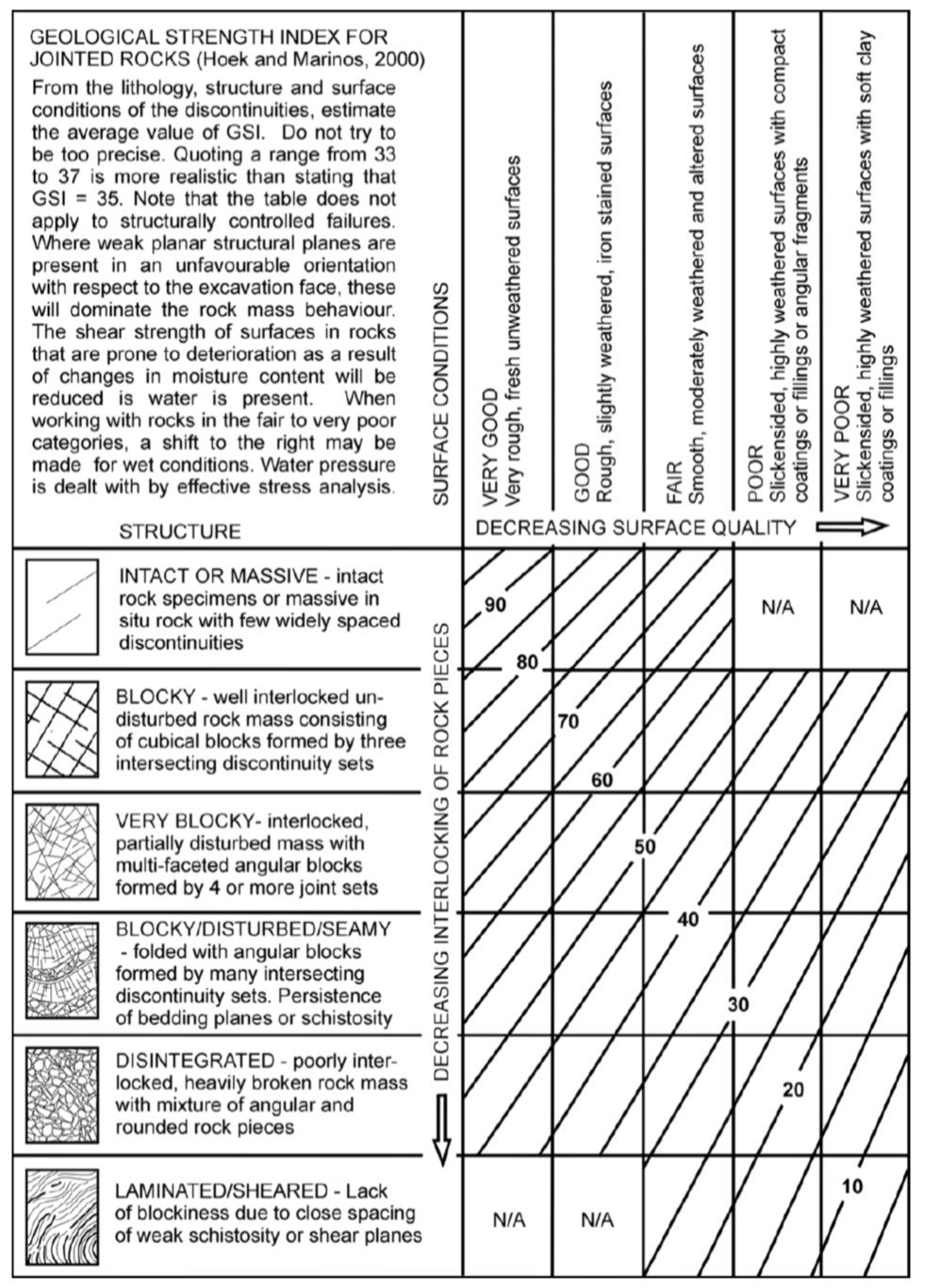
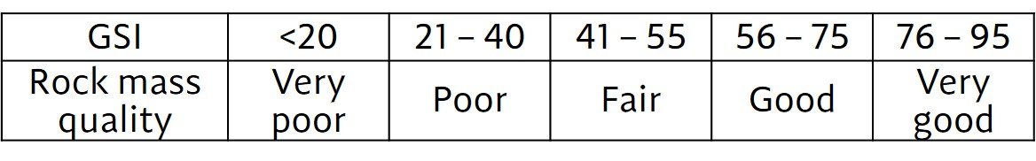
Table 2. Relation between GSI and rock mass quality.
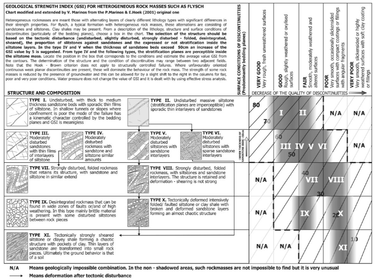
The GSI system has evolved substantially and nowadays there are several charts available for specific types of rock masses. Each of the individual GSI charts describes a particular rock mass type in greater detail than the general chart. For example, Figure 6 is a GSI chart for heterogeneous rock masses, especially flysch, proposed by Marinos (2017).
To quote one modification proposed by Marinos, the GSI values were increased from 10 to 35 units for the “Blocky” to “Undisturbed” structures, respectively, particularly for the siltstone type. Other GSI charts have been published to cover ophiolites (Marinos et al., 2005) and tectonically undisturbed molassic rocks (Hoek et al., 2005) encountered in northern Greece.
he GSI system was developed to deal with rock masses comprised of interlocking angular blocks in which the failure process is dominated by block sliding and rotation without a great deal of intact rock failure. Importantly, Hoek (2018) notes that the original purpose of the GSI chart was to provide a guide for the initial estimation of rock mass properties. It was always assumed that the user would improve the initial estimates with more detailed site investigations, numerical analyses, and back analyses of the tunnel or slope performance to validate or modify these estimates.
The GSI should not be used in cases where there are only one or two sets of discontinuities. Great caution should be taken when applying the method to blocky rock mass with minimal anisotropy. The application of GSI is also questionable in deep mining engineering systems, say more than 1000-m deep or so, in which the rock mass structure is so tight and under such a high stress field that its condition approaches that of intact rock. In such a structure, the GSI approaches 100 and the application of the classification system in the estimation of rock mass deformation and strength is no longer meaningful (Zuo and Shen, 2020).
Figure 6. GSI chart for heterogeneous rock masses with emphasis on flysch. After Marinos (2017).
3.2. The blast damage factor D
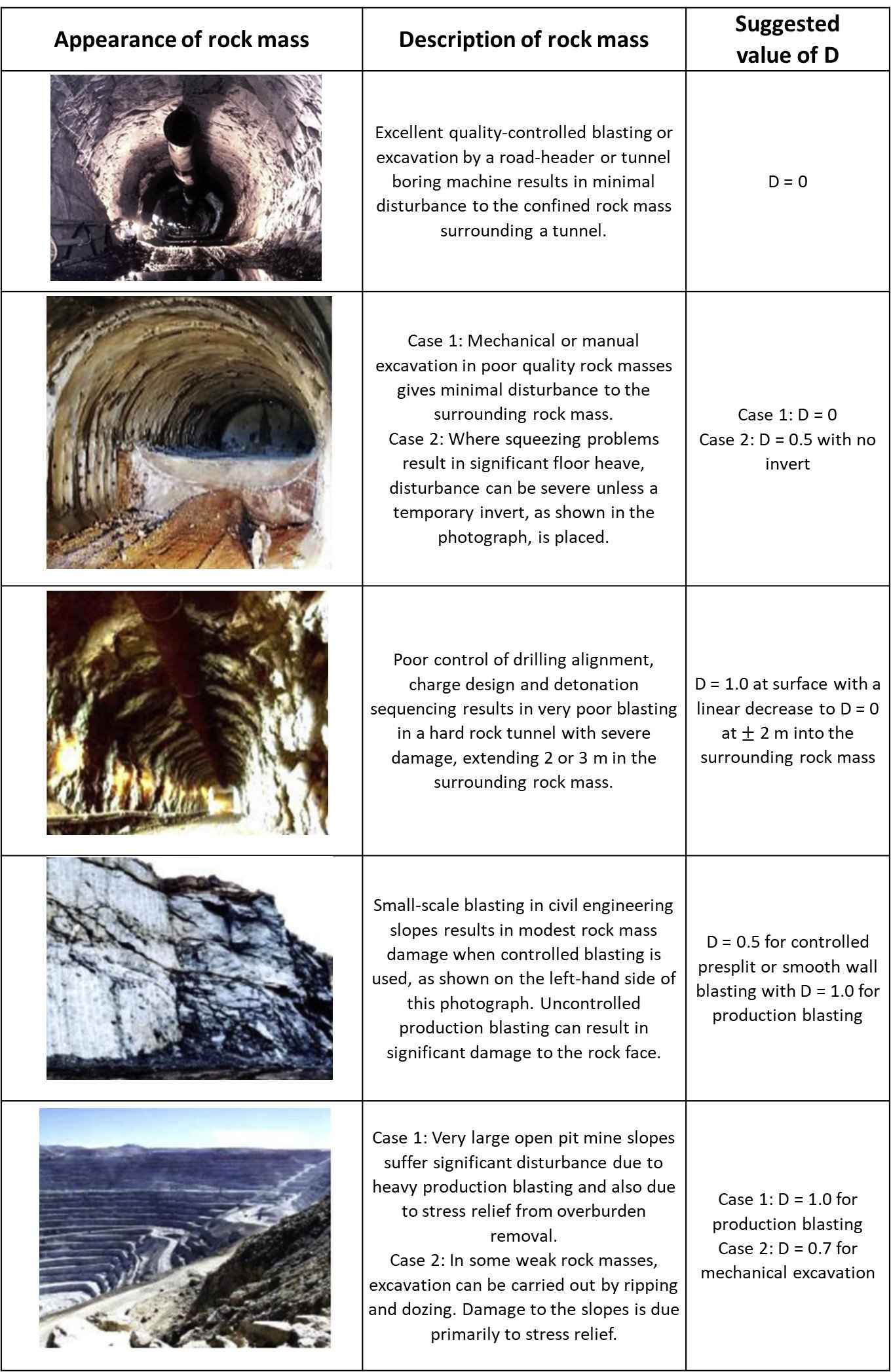
Then there’s the blast damage factor D. Practical experience in the design of rock slope projects has demonstrated that the estimated rock mass strength of a given slope is affected by the blast damage in slope excavations. In order to improve the accuracy of rock mass strength prediction under blast conditions, factor D, also known as the disturbance factor, was introduced in the generalized Hoek-Brown failure criterion. The value of D ranges from zero for undisturbed rock masses to unity for highly disturbed rock masses as caused by blast damage and stress relief. Hoek and Brown (2018) list five typical cases of engineering projects to illustrate how a D value can be selected. These cases are illustrated and described in Table 3. Importantly, Hoek (2018) notes that a single disturbance factor should not be applied to the entire rock mass surrounding an excavation.
Table 3. Five cases for determination of the blast damage factor D.
Wyllie (2018) notes that the influence of the blast damage factor D can be large. This is illustrated by a typical example in which
4. Relating the Hoek-Brown and Mohr-Coulomb failure criteria
Although the Hoek-Brown criterion has been around for a few decades now, many civil and mining engineers still prefer to rely on a linear Mohr-Coulomb failure envelope, perhaps because their first contact with geomechanical theory was with soils, a material traditionally modelled by a linear MC criterion, or maybe because the key variables in the MC approach – namely, the angle of internal friction and cohesion – are more intuitive than the corresponding variables in the Hoek-Brown framework. (Indeed, in the previous paragraph we ourselves have illustrated the relative effect of the blast damage factor D by quoting its effect on the friction angle
![\displaystyle {\phi }'={{\sin }^{{-1}}}\left[ {\frac{{6a{{m}_{b}}{{{\left( {s+{{m}_{b}}{{{{\sigma }'}}_{{3n}}}} \right)}}^{{a-1}}}}}{{2\left( {1+a} \right)\left( {2+a} \right)+6a{{m}_{b}}{{{\left( {s+{{m}_{b}}{{{{\sigma }'}}_{{3n}}}} \right)}}^{{a-1}}}}}} \right]\,\,\,(15)](https://s0.wp.com/latex.php?latex=%5Cdisplaystyle+%7B%5Cphi+%7D%27%3D%7B%7B%5Csin+%7D%5E%7B%7B-1%7D%7D%7D%5Cleft%5B+%7B%5Cfrac%7B%7B6a%7B%7Bm%7D_%7Bb%7D%7D%7B%7B%7B%5Cleft%28+%7Bs%2B%7B%7Bm%7D_%7Bb%7D%7D%7B%7B%7B%7B%5Csigma+%7D%27%7D%7D_%7B%7B3n%7D%7D%7D%7D+%5Cright%29%7D%7D%5E%7B%7Ba-1%7D%7D%7D%7D%7D%7B%7B2%5Cleft%28+%7B1%2Ba%7D+%5Cright%29%5Cleft%28+%7B2%2Ba%7D+%5Cright%29%2B6a%7B%7Bm%7D_%7Bb%7D%7D%7B%7B%7B%5Cleft%28+%7Bs%2B%7B%7Bm%7D_%7Bb%7D%7D%7B%7B%7B%7B%5Csigma+%7D%27%7D%7D_%7B%7B3n%7D%7D%7D%7D+%5Cright%29%7D%7D%5E%7B%7Ba-1%7D%7D%7D%7D%7D%7D+%5Cright%5D%5C%2C%5C%2C%5C%2C%2815%29&bg=ffffff&fg=000&s=1&c=20201002)
![\displaystyle {c}'=\frac{{{{\sigma }_{{ci}}}\left[ {\left( {1+2a} \right)s+\left( {1-a} \right){{m}_{b}}{{{{\sigma }'}}_{{3n}}}} \right]{{{\left( {s+{{m}_{b}}{{{{\sigma }'}}_{{3n}}}} \right)}}^{{a-1}}}}}{{\left( {1+a} \right)\left( {2+a} \right)\sqrt{{1+{{\left[ {6a{{m}_{b}}{{{\left( {s+{{m}_{b}}{{{{\sigma }'}}_{{3n}}}} \right)}}^{{a-1}}}} \right]}}/{{\left[ {\left( {1+a} \right)\left( {2+a} \right)} \right]}}\;}}}}\,\,\,(16)](https://s0.wp.com/latex.php?latex=%5Cdisplaystyle+%7Bc%7D%27%3D%5Cfrac%7B%7B%7B%7B%5Csigma+%7D_%7B%7Bci%7D%7D%7D%5Cleft%5B+%7B%5Cleft%28+%7B1%2B2a%7D+%5Cright%29s%2B%5Cleft%28+%7B1-a%7D+%5Cright%29%7B%7Bm%7D_%7Bb%7D%7D%7B%7B%7B%7B%5Csigma+%7D%27%7D%7D_%7B%7B3n%7D%7D%7D%7D+%5Cright%5D%7B%7B%7B%5Cleft%28+%7Bs%2B%7B%7Bm%7D_%7Bb%7D%7D%7B%7B%7B%7B%5Csigma+%7D%27%7D%7D_%7B%7B3n%7D%7D%7D%7D+%5Cright%29%7D%7D%5E%7B%7Ba-1%7D%7D%7D%7D%7D%7B%7B%5Cleft%28+%7B1%2Ba%7D+%5Cright%29%5Cleft%28+%7B2%2Ba%7D+%5Cright%29%5Csqrt%7B%7B1%2B%7B%7B%5Cleft%5B+%7B6a%7B%7Bm%7D_%7Bb%7D%7D%7B%7B%7B%5Cleft%28+%7Bs%2B%7B%7Bm%7D_%7Bb%7D%7D%7B%7B%7B%7B%5Csigma+%7D%27%7D%7D_%7B%7B3n%7D%7D%7D%7D+%5Cright%29%7D%7D%5E%7B%7Ba-1%7D%7D%7D%7D+%5Cright%5D%7D%7D%2F%7B%7B%5Cleft%5B+%7B%5Cleft%28+%7B1%2Ba%7D+%5Cright%29%5Cleft%28+%7B2%2Ba%7D+%5Cright%29%7D+%5Cright%5D%7D%7D%5C%3B%7D%7D%7D%7D%5C%2C%5C%2C%5C%2C%2816%29&bg=ffffff&fg=000&s=1&c=20201002)
where 

Figure 7. Nonlinear Mohr envelope for fractured rock mass defined by equations (15) and (16); best fit line shows cohesion and friction angle for applicable slope height. Rock mass parameters: uniaxial compressive strength 
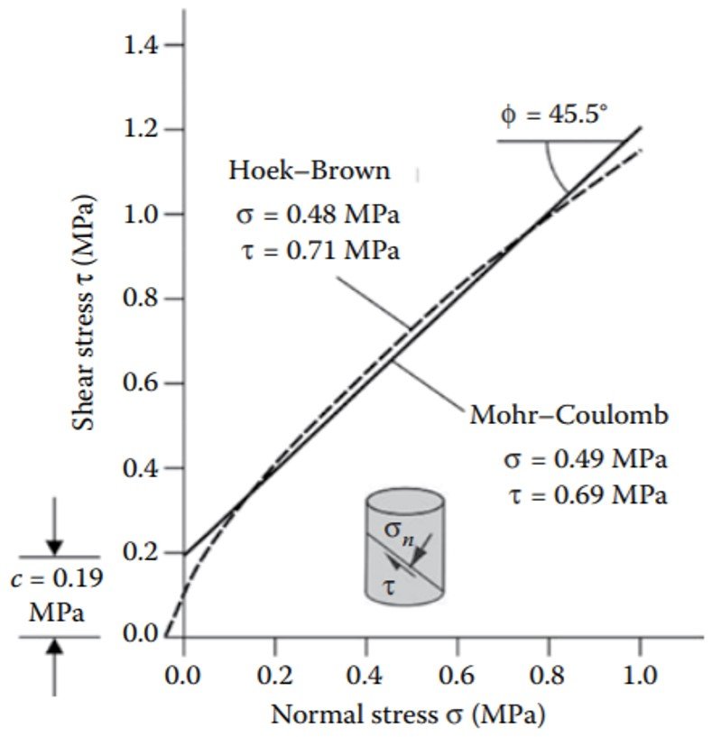
A conversion from a Hoek-Brown to a Mohr-Coulomb framework can be easily done with Rocscience’s RocLab software package. It should be observed that, albeit simple, this shift between criteria is prone to yield dangerously inaccurate values of friction angle and cohesion, especially when the range of minor stresses considered is not well thought out (Brown, 2008). Hoek’s Practical Rock Engineering ebook recommends that, where possible, the Hoek-Brown criterion should be applied directly.
References
Download references list here.