Murray’s Law and the Analysis of Arterial Bifurcations

Since blood vessels bifurcate multiple times before becoming capillaries, investigating an optimal pattern of bifurcation becomes an attractive task. Analyses of this sort have been undertaken for centuries; two contributions of seminal importance are the 1808 Croonian Lecture by Thomas Young and a 1926 paper by C. D. Murray that went largely unnoticed for decades. The discussion in this article closely follows the textbook of legendary biomechanicist Y. C. Fung, who passed away in December 2019, precisely two months after his 100th birthday. His Biomechanics: Circulation was published in the 1990s and remains the definitive textbook on biofluid mechanics.

1. Analysis of an Arterial Bifurcation

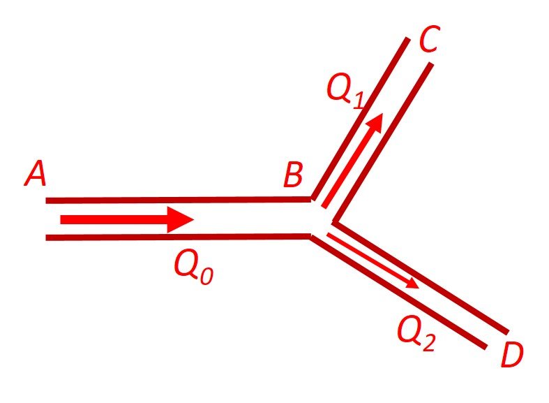
In our arterial bifurcation model, we propose a system of three cylindrical vessels, a main vessel AB and two daughter vessels BC and BD, as shown in Figure 1. A steady blood flow $\displaystyle {{Q}_{0}}$ is conveyed by the main vessel and then divides into a flow $\displaystyle {{Q}_{1}}$ into BC and a flow $\displaystyle {{Q}_{2}}$ into BD; needless to say, $\displaystyle {{Q}_{0}}$ = $\displaystyle {{Q}_{1}}$ + $\displaystyle {{Q}_{2}}$ . In our simple optimization task, points A, C and D will be fixed, but the location of B and the vessel radii are left for the designer to choose. Then, one may ask: is there an optimal position for the point B?

Figure 1. Arterial bifurcation model.

To provide a mathematical theory of bifurcations involving blood vessels, Murray suggested that the inner radius a of a blood vessel arises as an outcome of a “compromise” between the advantage of increasing the lumen, which decreases the resistance to flow, and the disadvantage of increasing overall blood volume, which increases the metabolic demand to maintain the blood. With this in mind, he proposed a cost function constituted of two terms. The first term is the rate at which work is done on the blood, which is given by the product of flow rate and pressure drop, $\displaystyle Q\Delta p$ . The second term is the rate at which energy is used up by the blood vessel by metabolism, which may be assumed to equal the volume of the blood vessel, $\displaystyle \pi {{a}^{2}}L$ , multiplied by some constant K. Accordingly, the cost function f becomes

$\displaystyle f=Q\Delta p+K\pi {{a}^{2}}L\,\,\,(\text{I})$

Replacing Q with Poiseuille’s law yields

$\displaystyle f=\frac{{8\mu L}}{{\pi {{a}^{4}}}}{{Q}^{2}}+K\pi {{a}^{2}}L\,\,\,(\text{II})$

For a given vessel of flow Q and length L, there must be some optimal radius, which can be obtained by differentiating the cost function, setting it to zero, and solving for a; that is,

$\displaystyle \frac{{df}}{{da}}=-\frac{{32\mu L{{Q}^{2}}}}{\pi }{{a}^{{-5}}}+2K\pi La=0$

$\displaystyle \therefore 2K\pi La=\frac{{32\mu L{{Q}^{2}}}}{\pi }{{a}^{{-5}}}$

$\displaystyle \therefore K\pi L{{a}^{6}}=\frac{{16\mu L{{Q}^{2}}}}{\pi }$

$\displaystyle \therefore {{a}^{6}}=\frac{{16\mu {{Q}^{2}}}}{{K{{\pi }^{2}}}}$

$\displaystyle \therefore a={{\left( {\frac{{16\mu }}{{K{{\pi }^{2}}}}} \right)}^{{\frac{1}{6}}}}{{Q}^{{\frac{1}{3}}}}\,\,\,(\text{III})$

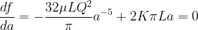
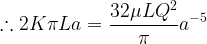
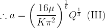
Clearly, the optimal radius of a blood vessel is proportional to blood flow to the 1/3 power. Substituting the result above into the cost function yields the minimum value of f,

$\displaystyle {{f}_{{\min }}}=\frac{{3\pi }}{2}KL{{a}^{2}}\,\,\,(\text{IV})$

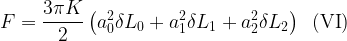
We can now turn to the design of the bifurcation pattern. The vessels are assigned radii and lengths as shown in Figure 2. The cost function of the entire system of blood vessels is the sum of the cost functions of individual vessel segments. Since the cost functions of all vessels are additive, we see at once that the vessels connecting A, C, and D in Figure 1 should be straight and lie in a plane (as this minimizes the length, L, when other things are fixed). The total cost function, which we denote by F, is then

$\displaystyle F=\frac{{3\pi K}}{2}\left( {a_{0}^{2}{{L}_{0}}+a_{1}^{2}{{L}_{1}}+a_{2}^{2}{{L}_{2}}} \right)\,\,\,(\text{V})$

Figure 2. Arterial bifurcation geometry.

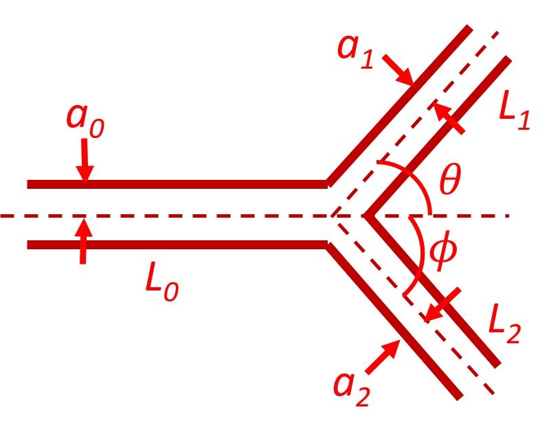
The lengths L₀, L₁, and L₂ are affected by the location of the point B – which, as the reader should recall, is the one point in the bifurcation that we are allowed to displace – and the radii a₀, a₁, and a₂ are related to the flows Q₀, Q₁, and Q₂ by equation (III). We proceed to minimize F by properly choosing the location of the bifurcation point B.

A small movement of B changes F by an amount F such that

$\displaystyle F=\frac{{3\pi K}}{2}\left( {a_{0}^{2}\delta {{L}_{0}}+a_{1}^{2}\delta {{L}_{1}}+a_{2}^{2}\delta {{L}_{2}}} \right)\,\,\,(\text{VI})$

An optimal location of B would make $\displaystyle \delta$ P = 0 for some arbitrary small movement of B. Let us consider three arbitrary small movements of B. First, let B move to B’ in the direction of AB, as shown in Figure 3.1. In this case,

$\displaystyle \delta {{L}_{0}}=\delta \,\,\,;\,\,\,\delta {{L}_{1}}=-\delta \cos \theta \,\,\,;\,\,\,\delta {{L}_{2}}=-\delta \cos \phi$

so that, substituting into equation (VI), we obtain

$\displaystyle \delta F=\frac{{3\pi K}}{2}\delta \left( {a_{0}^{2}-a_{1}^{2}\cos \theta -a_{2}^{2}\cos \phi } \right)$

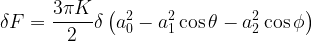
The optimum is obtained when

$\displaystyle a_{0}^{2}=a_{1}^{2}\cos \theta +a_{2}^{2}\cos \phi \,\,\,(\text{VII})$

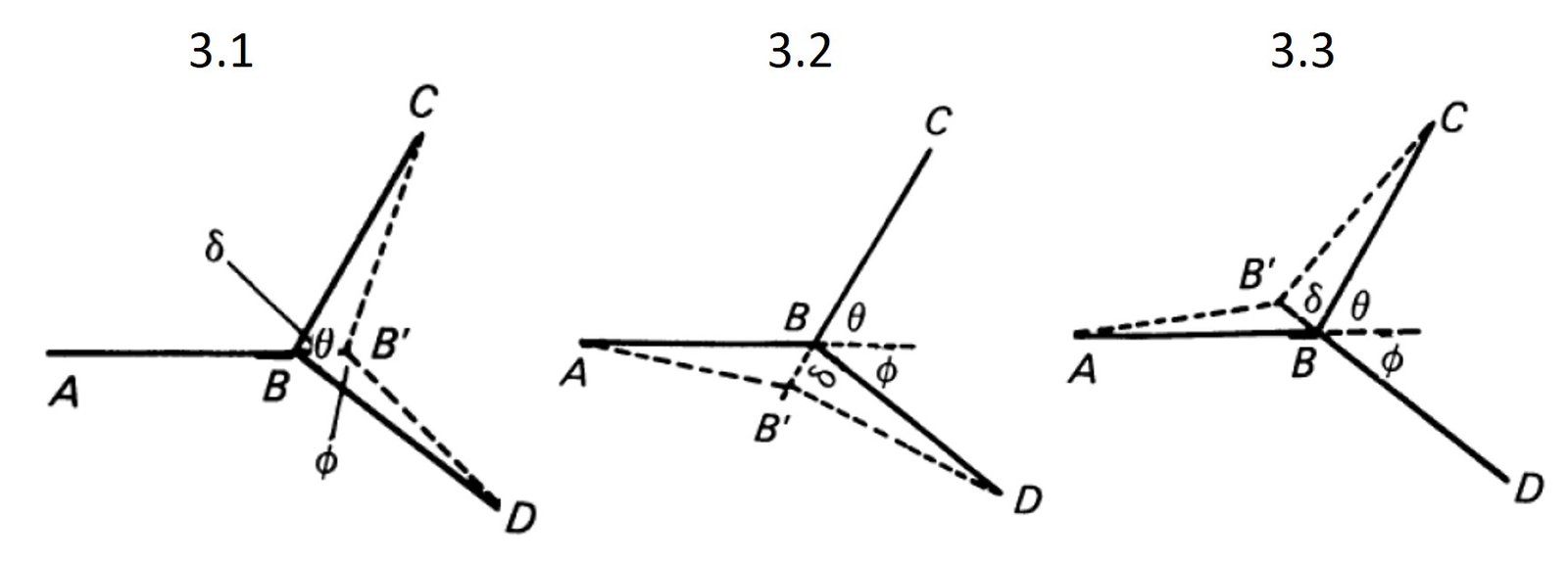
Next, let B move to B’ in the direction of CB, as shown in Figure 3.2. In this case,

$\displaystyle \delta {{L}_{0}}=-\delta \cos \theta \,\,\,;\,\,\,\delta {{L}_{1}}=\delta \,\,\,;\,\,\,\delta {{L}_{2}}=\delta \cos \left( {\theta +\phi } \right)$

so that

$\displaystyle \delta P=\frac{{3\pi K\delta }}{2}\left[ {-a_{0}^{2}\cos \theta +a_{1}^{2}+a_{2}^{2}\cos \left( {\theta +\phi } \right)} \right]$

The optimum condition is then

$\displaystyle -a_{0}^{2}\cos \theta +a_{1}^{2}+a_{2}^{2}\cos \left( {\theta +\phi } \right)=0\,\,\,(\text{VIII})$

Finally, let B move a short distance $\displaystyle \delta$ in the direction of DB, as shown in Figure 3.3. The optimal condition is, in this case, is

$\displaystyle -a_{0}^{2}\cos \phi +a_{1}^{2}\cos \left( {\theta +\phi } \right)+a_{2}^{2}=0\,\,\,(\text{IX})$

Figures 3.1-3. Small bifurcation displacements.

Gleaning equations (VII), (VIII), and (IX), we have

$\displaystyle a_{0}^{2}=a_{1}^{2}\cos \theta +a_{2}^{2}\cos \phi$

$\displaystyle -a_{0}^{2}\cos \theta +a_{1}^{2}+a_{2}^{2}\cos \left( {\theta +\phi } \right)=0$

$\displaystyle -a_{0}^{2}\cos \phi +a_{1}^{2}\cos \left( {\theta +\phi } \right)+a_{2}^{2}=0$

These equations can be solved for the cosines by means of the Mathematica code

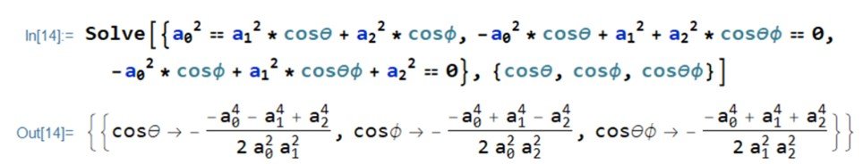
That is,

$\displaystyle \cos \theta =\frac{{a_{0}^{4}+a_{1}^{4}-a_{2}^{4}}}{{2a_{0}^{2}a_{1}^{2}}}\,\,\,(\text{X})$

$\displaystyle \cos \phi =\frac{{a_{0}^{4}-a_{1}^{4}+a_{2}^{4}}}{{2a_{0}^{2}a_{2}^{2}}}\,\,\,(\text{XI})$

$\displaystyle \cos \left( {\theta +\phi } \right)=\frac{{a_{0}^{4}-a_{1}^{4}-a_{2}^{4}}}{{2a_{1}^{2}a_{2}^{2}}}\,\,\,(\text{XII})$

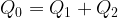
From conservation of mass, we can write

$\displaystyle {{Q}_{0}}={{Q}_{1}}+{{Q}_{2}}$

which, combined with equation (III), yields

$\displaystyle a_{0}^{3}=a_{1}^{3}+a_{2}^{3}\,\,\,(\text{XIII})$

This result is known as Murray’s law. We can isolate a₂ and write

$\displaystyle {{a}_{2}}={{\left( {a_{0}^{3}-a_{1}^{3}} \right)}^{{{1}/{3}\;}}}$

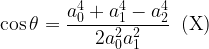
Then, we substitute a₂ into equation (X) to give

$\displaystyle \cos \theta =\frac{{a_{0}^{4}+a_{1}^{4}-{{{\left( {a_{0}^{3}-a_{1}^{3}} \right)}}^{{{4}/{3}\;}}}}}{{2a_{0}^{2}a_{1}^{2}}}\,\,\,(\text{XIV})$

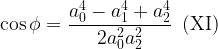
The cosine of one of the angles outlined by the bifurcation has been expressed in terms of two vessel radii only. The same can be done for cos $\displaystyle \phi$ ,

$\displaystyle \cos \phi =\frac{{a_{0}^{4}-{{{\left( {a_{0}^{3}-a_{2}^{3}} \right)}}^{{{4}/{3}\;}}}+a_{2}^{4}}}{{2a_{0}^{2}a_{2}^{2}}}\,\,\,(\text{XV})$

and finally for cos( $\displaystyle \theta$ + $\displaystyle \phi$ ),

$\displaystyle \cos \left( {\theta +\phi } \right)=\frac{{{{{\left( {a_{1}^{3}+a_{2}^{3}} \right)}}^{{{4}/{3}\;}}}-a_{1}^{4}-a_{2}^{4}}}{{2a_{1}^{2}a_{2}^{2}}}\,\,(\text{XVI})$

Using these expressions, we can draw some interesting conclusions regarding the geometry of the bifurcation under special circumstances.

2. If the radii of the daughter branches are equal, the bifurcating angles are equal

To show this, let a₁ = a₂. Substituting into equation (XIV) brings to

$\displaystyle \cos \theta =\frac{{a_{0}^{4}+a_{1}^{4}-{{{\left( {a_{0}^{3}-a_{1}^{3}} \right)}}^{{{4}/{3}\;}}}}}{{2a_{0}^{2}a_{1}^{2}}}=\frac{{a_{0}^{4}+a_{2}^{4}-{{{\left( {a_{0}^{3}-a_{2}^{2}} \right)}}^{{{4}/{3}\;}}}}}{{2a_{0}^{2}a_{2}^{2}}}\,\,\,(\text{XVII})$

The rightmost side of this result happens to have the same form as equation (XV). Thus,

$\displaystyle \cos \theta =\cos \phi$

which means that

$\displaystyle \theta =\phi$

Simply put, if the radii of the daughter branches are equal, the bifurcation angles will be equal.

3. If a₂ $\displaystyle \gg$ a₁, then a₂ = a₀ and $\displaystyle \phi$ = $\displaystyle \pi$ /2

At this point, we assume that the radius of one daughter vessel is much larger than the other. We can rewrite equation (XVI) as

$\displaystyle \cos \left( {\theta +\phi } \right)=\frac{{{{{\left( {a_{1}^{3}+a_{2}^{3}} \right)}}^{{4/3}}}-a_{1}^{4}-a_{2}^{4}}}{{2a_{1}^{2}a_{2}^{2}}}=\frac{{{{{\left( {a_{1}^{3}+a_{2}^{3}} \right)}}^{{4/3}}}-(a_{1}^{4}+a_{2}^{4})}}{{2a_{1}^{2}a_{2}^{2}}}$

If one radius is indeed much greater than the other, we must have $\displaystyle a_{1}^{3}$ + $\displaystyle a_{2}^{3}$ $\displaystyle \approx$ $\displaystyle a_{2}^{3}$ and $\displaystyle a_{1}^{4}$ + $\displaystyle a_{2}^{4}$ $\displaystyle \approx$ $\displaystyle a_{2}^{4}$ , so that

$\displaystyle \cos \left( {\theta +\phi } \right)=\frac{{{{{\left( {a_{1}^{3}+a_{2}^{3}} \right)}}^{{4/3}}}-(a_{1}^{4}+a_{2}^{4})}}{{2a_{1}^{2}a_{2}^{2}}}\approx \frac{{{{{\left( {a_{2}^{3}} \right)}}^{{{4}/{3}\;}}}-a_{2}^{4}}}{{2a_{1}^{2}a_{2}^{2}}}=0$

Then, from elementary trigonometry,

$\displaystyle \theta +\phi =\arccos 0\to \theta +\phi =\frac{\pi }{2}$

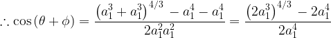
Similarly, consider the equation obtained for cos $\displaystyle \theta$ ,

$\displaystyle \cos \theta =\frac{{a_{0}^{4}+a_{1}^{4}-{{{\left( {a_{0}^{3}-a_{1}^{3}} \right)}}^{{{4}/{3}\;}}}}}{{2a_{0}^{2}a_{1}^{2}}}$

Here, $\displaystyle a_{0}^{4}$ + $\displaystyle a_{1}^{4}$ $\displaystyle \approx$ $\displaystyle a_{0}^{4}$ and $\displaystyle a_{0}^{3}$ – $\displaystyle a_{1}^{3}$ $\displaystyle \approx$ $\displaystyle a_{0}^{3}$ , giving

$\displaystyle \cos \theta =\frac{{a_{0}^{4}+a_{1}^{4}-{{{\left( {a_{0}^{3}-a_{1}^{3}} \right)}}^{{{4}/{3}\;}}}}}{{2a_{0}^{2}a_{1}^{2}}}\approx \frac{{a_{0}^{4}-{{{\left( {a_{0}^{3}} \right)}}^{{{4}/{3}\;}}}}}{{2a_{0}^{2}a_{1}^{2}}}=0$

$\displaystyle \therefore \theta =\frac{\pi }{2}$

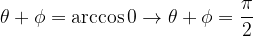
or 90^o. Finally, noting that $\displaystyle \theta$ + $\displaystyle \phi$ = $\displaystyle \pi$ /2 brings to

$\displaystyle \theta +\phi =\frac{\pi }{2}\to \frac{\pi }{2}+\phi =\frac{\pi }{2}$

$\displaystyle \therefore \phi =0$

These results show that, when the radius of one of the daughter vessels is much greater than that of the other, the bifurcation approaches a T shape.

4. When a₁ = a₂, it follows that a₁/a₀ = 2^-1/3 = 0.794 and cos $\displaystyle \theta$ = 0.794. Thus, $\displaystyle \theta$ = 37.5^o

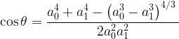
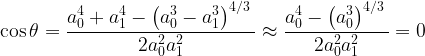
Here, we posit that the two daughter vessels have the same radius. Substituting a₁ = a₂ into equation (XVI) brings to

$\displaystyle \cos \left( {\theta +\phi } \right)=\frac{{{{{\left( {a_{1}^{3}+a_{2}^{3}} \right)}}^{{{4}/{3}\;}}}-a_{1}^{4}-a_{2}^{4}}}{{2a_{1}^{2}a_{2}^{2}}}$

$\displaystyle \therefore \cos \left( {\theta +\phi } \right)=\frac{{{{{\left( {a_{1}^{3}+a_{1}^{3}} \right)}}^{{{4}/{3}\;}}}-a_{1}^{4}-a_{1}^{4}}}{{2a_{1}^{2}a_{1}^{2}}}=\frac{{{{{\left( {2a_{1}^{3}} \right)}}^{{{4}/{3}\;}}}-2a_{1}^{4}}}{{2a_{1}^{4}}}$

$\displaystyle \therefore \cos \left( {\theta +\phi } \right)=\frac{{a_{1}^{4}\left( {{{2}^{{{4}/{3}\;}}}-2} \right)}}{{2a_{1}^{4}}}$

$\displaystyle \therefore \cos \left( {\theta +\phi } \right)=0.2599$

However, we established in Part 2 that $\displaystyle \theta$ = $\displaystyle \phi$ when a₁ = a₂. Accordingly,

$\displaystyle \cos \left( {\theta +\phi } \right)=0.2599\to \cos 2\theta =0.2599$

$\displaystyle \therefore \theta =\frac{1}{2}\arccos \left( {0.2599} \right)\approx 37.5{}^\text{o}$

and, consequently, $\displaystyle \phi$ = 37.5^o as well. Fung notes that, when a₁ = a₂, we have a₁/a₀ = 2^-1/3 = 0.794, thus $\displaystyle \theta$ = 37.5^o.

Let a₀ denote the radius of the aorta, and assume equal bifurcation in all generations. Thus, the radius of the first generation is 0.794a₀, the radius of the second generation is 0.794²a₀, and, in general terms, that of the n-th generation is given by

$\displaystyle {{a}_{n}}={{\left( {0.794} \right)}^{n}}{{a}_{0}}$

Substituting a_n = 5 $\displaystyle \times$ 10^-4 cm and a₀ = 1.5 cm in the foregoing expression, we have

$\displaystyle 5\times {{10}^{{-4}}}={{\left( {0.794} \right)}^{n}}\times 1.5$

This equation can be solved using logarithms to yield n = 34.7 $\displaystyle \approx$ 35. That is, about 35 generations of equal bifurcations are necessary to reduce the size of the blood vessels from the aorta to the smallest capillary. Since each generation multiplies the number of vessels by 2, the total number of blood vessels is 2³⁵ $\displaystyle \approx$ 3.44 $\displaystyle \times$ 10¹⁰, or about 34 billion conduits. However, the symmetry we assumed cannot be taken too seriously, as there is only one symmetric bifurcation in humans, and none in the dog.

In the early 19th century, Thomas Young took arbitrary dimensions for the aorta and capillaries and proposed a model for the successive ramifications of blood vessels. Young chose a symmetrical, dichotomous system in which the diameter of each branch was “about 4/5 of that of the trunk, or more accurately 1:2^1/3.“ By assuming this geometric ratio between the diameters of daughter and parent vessels, Young calculated that 29 bifurcations were necessary to diminish the aorta to the size of the capillaries. This estimate is not too much far off from ours. From estimates of the lengths of the aorta and the capillaries, Young constructed a geometric series for lengths of the approximately thirty generations of vessels and went on to calculate blood volumes, velocities of flow, and resistances in the different stages of the system. Young does not say why he chose a ratio of 2^1/3:1, but it seems certain that he was familiar with a rule – either empirical or theoretical – that favored his choice.

References

• FUNG, Y. (1997). Biomechanics: Circulation. 2nd edition. Berlin/Heidelberg: Springer.

• HUMPHREY, J. and DELANGE, S. (2004). An Introduction to Biomechanics. Berlin/Heidelberg: Springer.

• VOGEL, S. (1992). Vital Circuits. Oxford: Oxford University Press.

Murray’s Law and the Analysis of Arterial Bifurcations

Subscribe to our Mailing List!

Featured Posts

A Primer on NAND Flash Memories

Solidification Time and Chvorinov’s Rule

Step-Growth Polymerization, the Carothers Equation, and the Flory-Schulz Distribution

More Articles

Vertical-Axis Wind Turbines

Shock Wave-Boundary Layer Interaction: Upstream and Downstream Mechanisms

Fields of Study

More

© 2024 Montogue Quiz

Subscribe to
our Mailing List!

Subscribe to our Mailing List!

Subscribe to receive our latest materials in your inbox.

Homework Help

© 2024 Montogue Quiz

Subscribe to our Mailing List!