Prandtl-Meyer Expansion Waves: Derivation and Problems

1. Introduction

Oblique shock waves occur when supersonic flow is turned into itself. In contrast, when a supersonic flow is turned away from itself along a convex corner, an expansion fan is formed, as illustrated in Figure 1.

Figure 1. Expansion fan.

The expansion fan is a continuous expansion region that can be visualized as an infinite number of Mach waves, each making a Mach angle $\displaystyle \mu$ with the local flow direction. The expansion fan is bounded upstream by a Mach wave which makes the angle $\displaystyle {{\mu }_{1}}$ with respect to the upstream flow such that $\displaystyle {{\mu }_{1}}$ = arcsin(1/M₁), where M₁ is the normal Mach number of flow upstream of the fan. The expansion fan is bounded downstream by another Mach wave, in this case one that makes an angle $\displaystyle {{\mu }_{2}}$ with respect to the downstream flow such that $\displaystyle {{\mu }_{2}}$ = arcsin(1/M₂), where M₂ is the normal Mach number of flow just downstream of the fan. Thus, the expansion can be visualized as a continuous succession of Mach waves; since Mach waves are isentropic, the expansion itself is also isentropic. This is in direct contrast to flow across an oblique shock, which is always accompanied by some entropy increase.

An expansion fan emanating from a sharp convex corner is called a Prandtl-Meyer expansion wave, so named in honor of Ludwig Prandtl (1875 -1953) and Theodor Meyer (1882 – 1972). Prandtl is one of the most celebrated aerodynamicists of all time, known for his seminal contributions to the field in the first third of the 20th century. Meyer was a doctoral student of Prandtl’s at Göttingen University; his doctoral dissertation, published in 1908, laid the foundations of expansion wave theory.

2. Deriving the Prandtl-Meyer function

Figure 2. Expansion wave.

Let us turn to a mathematical treatment of expansion wave phenomena. Consider first a single Mach wave, expanding and deflecting the supersonic flow through a very small angle of magnitude $\displaystyle \theta$ = dv, as shown in Figure 2. With no pressure gradient in the tangential direction, again, there is no change of the tangential velocity component across the wave. Equating the expressions for V_t upstream and downstream of the Mach wave (Figure 2), we may write

$\displaystyle {{V}_{t}}=V\cos \mu$

$\displaystyle \therefore {{V}_{t}}=\left( {V+dV} \right)\cos \left( {\mu +dv} \right)$

$\displaystyle \therefore {{V}_{t}}=\left( {V+dV} \right)\left( {\cos dv\cos \mu -\sin dv\sin \mu } \right)\,\,\,(1)$

Since dv is a very small angle, we may employ the approximations cos dv $\displaystyle \approx$ 1 and sin dv $\displaystyle \approx$ dv, so that equation (1) can be restated as

$\displaystyle V\cos \mu =\left( {V+dV} \right)\left( {\cos \mu -\sin \mu \,dv} \right)\,\,\,\left( 2 \right)$

Expanding the product on the right-hand side,

$\displaystyle V\cos \mu =V\cos \mu -V\sin \mu \,dv+\,\cos \mu \,dV-\sin \mu \,dV\,dv\,\,\,(3)$

The last term on the RHS contains a product of differentials and can be neglected. Simplifying further leads to

$\displaystyle 0=-V\sin \mu \,dv+\,\cos \mu \,dV$

$\displaystyle \therefore \frac{{dV}}{V}=\left( {\tan \mu } \right)dv\,\,\,(4)$

Since sin $\displaystyle \mu$ = 1/M, we may write

$\displaystyle \tan \mu =\frac{{\sin \mu }}{{\cos \mu }}=\frac{{\sin \mu }}{{\sqrt{{1-{{{\sin }}^{2}}\mu }}}}=\frac{1}{{\sqrt{{{{M}^{2}}-1}}}}\,\,\,(5)$

Substituting in (4),

$\displaystyle \frac{{dV}}{V}=\left( {\tan \mu } \right)dv=\frac{1}{{\sqrt{{{{M}^{2}}-1}}}}dv\,\,\,(6)$

As in the mathematical treatment of oblique shocks, our aim is to express the variation of flow properties as a function of turning angle and Mach number only. From the definition of Mach number for a perfect gas with constant specific heats, we may write

$\displaystyle V=M\sqrt{{\gamma RT}}\,\,\,(7)$

Taking the logarithm of each side and differentiating,

$\displaystyle \frac{{dV}}{V}=\frac{{dM}}{M}+\frac{1}{2}\frac{{dT}}{T}\,\,\,(8)$

However, for this adiabatic flow, there is no change in stagnation temperature. Therefore, denoting stagnation conditions with a “o” subscript and using an elementary compressible flow relation,

$\displaystyle {{T}_{o}}=\text{constant}=T\left( {1+\frac{{\gamma -1}}{2}{{M}^{2}}} \right)\,\,\,(9)$

Taking the logarithm and differentiating,

$\displaystyle 0=\frac{{dT}}{T}+\frac{{\left( {\gamma -1} \right)MdM}}{{1+\frac{{\gamma -1}}{2}{{M}^{2}}}}\,\,\,(10)$

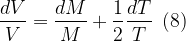
Equations (8) and (10) can be combined to yield

$\displaystyle \frac{{dV}}{V}=\frac{{dM}}{M}-\frac{1}{2}\left[ {\frac{{\left( {\gamma -1} \right)MdM}}{{1+\frac{{\gamma -1}}{2}{{M}^{2}}}}} \right]\,\,\,(11)$

$\displaystyle \frac{{dV}}{V}=\left( {\frac{1}{{1+\frac{{\gamma -1}}{2}{{M}^{2}}}}} \right)\frac{{dM}}{M}\,\,\,(12)$

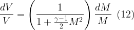
Substituting into (6) yields

$\displaystyle dv=\left( {\frac{{\sqrt{{{{M}^{2}}-1}}}}{{1+\frac{{\gamma -1}}{2}{{M}^{2}}}}} \right)\frac{{dM}}{M}\,\,\,(13)$

Now, let

$\displaystyle {{x}^{2}}={{M}^{2}}-1\,\,\,(14)$

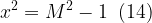
or, equivalently, M² = 1 + x². It follows that 2MdM = 2xdx, or

$\displaystyle \frac{{dM}}{M}=\frac{{xdx}}{{1+{{x}^{2}}}}\,\,\,(15)$

Using the relation above and identity (14), we substitute into (13) to obtain

$\displaystyle dv=\left( {\frac{{\sqrt{{{{M}^{2}}-1}}}}{{1+\frac{{\gamma -1}}{2}{{M}^{2}}}}} \right)\frac{{dM}}{M}=\frac{x}{{1+\frac{{\gamma -1}}{2}\left( {1+{{x}^{2}}} \right)}}\frac{{xdx}}{{1+{{x}^{2}}}}$

$\displaystyle \therefore dv=\frac{{2{{x}^{2}}}}{{\left( {\gamma +1} \right)+\left( {\gamma -1} \right){{x}^{2}}}}\left( {\frac{1}{{1+{{x}^{2}}}}} \right)dx\,\,\,(16)$

Next, use partial fractions to divide the right-hand side into two groups of terms,

$\displaystyle \frac{A}{{\left( {\gamma +1} \right)+\left( {\gamma -1} \right){{x}^{2}}}}+\frac{B}{{1+{{x}^{2}}}}=\frac{{2{{x}^{2}}}}{{\left[ {\left( {\gamma +1} \right)+\left( {\gamma -1} \right){{x}^{2}}} \right]\left( {1+{{x}^{2}}} \right)}}\,\,\,(17)$

so that

$\displaystyle A+A{{x}^{2}}+\left( {\gamma +1} \right)B+\left( {\gamma -1} \right)B{{x}^{2}}=2{{x}^{2}}\,\,\,(18)$

Equating the two sides yields the equations

$\displaystyle A+\left( {\gamma -1} \right)B=2\,\,\,(19)$

$\displaystyle A+\left( {\gamma +1} \right)B=0\,\,\,(20)$

Solving this system of equations yields A = $\displaystyle \gamma$ + 1 and B = –1. Thus, the transformed equation can be arranged into two groups and leads to the following two integrals:

$\displaystyle -\int{{\left( {\frac{{\sqrt{{{{M}^{2}}-1}}}}{{1+\frac{{\gamma -1}}{2}{{M}^{2}}}}} \right)}}\frac{{dM}}{M}=-\int{{\frac{{\gamma +1}}{{\left( {\gamma +1} \right)+\left( {\gamma -1} \right){{x}^{2}}}}dx-\int{{\frac{1}{{1+{{x}^{2}}}}dx}}}}$

$\displaystyle \therefore -\int{{\left( {\frac{{\sqrt{{{{M}^{2}}-1}}}}{{1+\frac{{\gamma -1}}{2}{{M}^{2}}}}} \right)}}\frac{{dM}}{M}=-\int{{\frac{1}{{1+\left( {\frac{{\gamma -1}}{{\gamma +1}}} \right){{x}^{2}}}}dx-\int{{\frac{1}{{1+{{x}^{2}}}}dx}}}}\,\,\,(21)$

At this point, we evoke the tabulated integral

$\displaystyle \int{{\frac{{du}}{{{{a}^{2}}+{{b}^{2}}{{u}^{2}}}}}}=\frac{1}{{ab}}{{\tan }^{{-1}}}\left( {\frac{{bu}}{a}} \right)\,\,\,(22)$

which ultimately gives

$\displaystyle -\int{{\left( {\frac{{\sqrt{{{{M}^{2}}-1}}}}{{1+\frac{{\gamma -1}}{2}{{M}^{2}}}}} \right)}}\frac{{dM}}{M}=-\left\{ {\sqrt{{\frac{{\gamma +1}}{{\gamma -1}}}}{{{\tan }}^{{-1}}}\left[ {\sqrt{{\frac{{\gamma -1}}{{\gamma +1}}\left( {{{M}^{2}}-1} \right)}}} \right]-{{{\tan }}^{{-1}}}\left( {\sqrt{{{{M}^{2}}-1}}} \right)} \right\}\,\,\,(23)$

We can return to equation (13) with this relationship, integrating and finding the change of Mach number associated with the turning of a supersonic flow through a finite angle $\displaystyle \theta$ = v₂ – v₁,

$\displaystyle \theta =\int_{{{{v}_{1}}}}^{{{{v}_{2}}}}{{dv}}=\int_{{{{M}_{1}}}}^{{{{M}_{2}}}}{{\frac{{\sqrt{{{{M}^{2}}-1}}}}{{1+\left[ {{{\left( {\gamma -1} \right)}}/{2}\;} \right]{{M}^{2}}}}}}\frac{{dM}}{M}\,\,\,(24)$

Using (23),

$\displaystyle {{v}_{2}}-{{v}_{1}}=\left\{ {\sqrt{{\frac{{\gamma +1}}{{\gamma -1}}}}{{{\tan }}^{{-1}}}\left[ {\sqrt{{\frac{{\gamma -1}}{{\gamma +1}}\left( {{{M}^{2}}-1} \right)}}} \right]-{{{\tan }}^{{-1}}}\left( {\sqrt{{{{M}^{2}}-1}}} \right)} \right\}\,\,\,(25)$

For the purpose of tabulating this result, it is convenient to define a reference state such that M = M_ref at v_ref, giving

$\displaystyle v-{{v}_{{\text{ref}}}}=\left. {\left\{ {\sqrt{{\frac{{\gamma +1}}{{\gamma -1}}}}{{{\tan }}^{{-1}}}\left[ {\sqrt{{\frac{{\gamma -1}}{{\gamma +1}}\left( {{{M}^{2}}-1} \right)}}} \right]-{{{\tan }}^{{-1}}}\left( {\sqrt{{{{M}^{2}}-1}}} \right)} \right\}} \right|_{{{{M}_{{ref}}}}}^{M}\,\,\,(26)$

Letting the reference state be v = 0 at M = 1, we may write

$\displaystyle v\left( M \right)=\sqrt{{\frac{{\gamma +1}}{{\gamma -1}}}}{{\tan }^{{-1}}}\left[ {\sqrt{{\frac{{\gamma -1}}{{\gamma +1}}\left( {{{M}^{2}}-1} \right)}}} \right]-{{\tan }^{{-1}}}\left( {\sqrt{{{{M}^{2}}-1}}} \right)\,\,\,(27)$

The expression above, v(M), is known as the Prandtl-Meyer function. It represents the angle through which a stream, initially at Mach 1, must be expanded to reach a supersonic Mach number M. Importantly, the Prandtl-Meyer function is a monotonically increasing function of M.

Two limiting cases for v can be considered, namely M $\displaystyle \to$ 1 and M $\displaystyle \to$ $\displaystyle \infty$ . The former is elementary and yields v $\displaystyle \to$ 0. In the latter case, it can be shown that

$\displaystyle {{v}_{{\max }}}=\frac{\pi }{2}\left( {\sqrt{{\frac{{\gamma +1}}{{\gamma -1}}}}-1} \right)\,\,\,(28)$

The expression above yields the maximum turning angle for Prandtl-Meyer flow and clearly depends only on the ratio of specific heats. For air, $\displaystyle \gamma$ = 1.4 and v_max = 130.45^o. This maximum value is of academic interest only, since long before a supersonic flow is deflected through this angle the continuum assumption would become invalid as the static pressure attains very low values.

3. Problems involving expansion waves

To determine the angle through which a flow would have to be turned to expand from some upstream Mach number M₁ to some downstream Mach number M₂, with M₁ $\displaystyle \ne$ 1, one needs only subtract the PM function v₁ at M₁ from the value of v₂ at M₂. That is, the turning angle $\displaystyle \theta$ is related to the Prandtl-Meyer functions by the simple relationship

$\displaystyle \theta =v\left( {{{M}_{2}}} \right)-v\left( {{{M}_{1}}} \right)\,\,\,(29)$

Values of the PM function are tabulated in any gas dynamics textbook and can be found here. To solve a simple expansion wave problem, we may proceed as follows:

For the given M₁, obtain v(M₁) from the Prandtl-Meyer table.
Calculate v(M₂) from equation (29) using the known $\displaystyle \theta$ and the value of v(M₁) obtained in step 1.
Obtain M₂ from the expansion wave table corresponding to the value of v(M₂) from step 2.
The expansion wave is isentropic; hence, stagnation pressure p₀ and stagnation temperature T₀ are constant through the wave, that is, T_0,2 = T_0,1 and p_0,2 = p_0,1. The temperature ratio can then be written as

$\displaystyle \frac{{{{T}_{2}}}}{{{{T}_{1}}}}=\frac{{{{{{T}_{2}}}}/{{{{T}_{{0,2}}}}}\;}}{{{{{{T}_{1}}}}/{{{{T}_{{0,1}}}}}\;}}=\frac{{1+\left[ {{{\left( {\gamma -1} \right)}}/{2}\;} \right]M_{1}^{2}}}{{1+\left[ {{{\left( {\gamma -1} \right)}}/{2}\;} \right]M_{2}^{2}}}\,\,\,(30)$

If only T₂ interests you, use the isentropic flow relation

$\displaystyle {{T}_{2}}={{\left( {1+\frac{{\gamma -1}}{2}M_{2}^{2}} \right)}^{{-1}}}{{T}_{0}}\,\,\,(31)$

As for the pressure ratio,

$\displaystyle \frac{{{{p}_{2}}}}{{{{p}_{1}}}}=\frac{{{{{{p}_{2}}}}/{{{{p}_{0}}}}\;}}{{{{{{p}_{1}}}}/{{{{p}_{0}}}}\;}}={{\left\{ {\frac{{1+\left[ {{{\left( {\gamma -1} \right)}}/{2}\;} \right]M_{1}^{2}}}{{1+\left[ {{{\left( {\gamma -1} \right)}}/{2}\;} \right]M_{2}^{2}}}} \right\}}^{{{\gamma }/{{\left( {\gamma -1} \right)}}\;}}}\,\,\,(32)$

If only p₂ interests you, use the isentropic flow relation

$\displaystyle {{p}_{2}}={{\left( {1+\frac{{\gamma -1}}{2}M_{2}^{2}} \right)}^{{-\gamma /\left( {\gamma -1} \right)}}}{{p}_{0}}\,\,\,(33)$

Example problem 1

A uniform supersonic flow of air ( $\displaystyle \gamma$ = 1.4) at Mach 2.6, with stagnation pressure of 5 MPa and stagnation temperature of 1000 K, expands around a 20^o convex corner. Determine

the downstream Mach number;
the stagnation pressure and temperature;
the static pressure and temperature

Part 1: Entering a Mach number of 2.6 into the Prandtl-Meyer table, we read v(M₁) = 41.4147^o. Using this quantity and $\displaystyle \theta$ = 20^o, we write

$\displaystyle {{v}_{2}}={{v}_{1}}+\theta =41.4147{}^\text{o}+20{}^\text{o}=61.4147{}^\text{o}$

Entering this angle into the Prandtl-Meyer table, the closest data points we have are for v = 61.2990^o, which corresponds to M = 3.68, and for v = 61.5953^o, which corresponds to M = 3.70. As a rudimentary approximation, we interpolate linearly to obtain M₂ $\displaystyle \approx$ 3.688.

Part 2: Expansion waves are isentropic; it follows that the stagnation pressure remains unchanged at 5 MPa. Likewise, the stagnation temperature remains unchanged at 1000 K.

Part 3: To compute the static pressure, we appeal to equation (33),

$\displaystyle {{p}_{2}}={{\left( {1+\frac{{\gamma -1}}{2}M_{2}^{2}} \right)}^{{-\gamma /\left( {\gamma -1} \right)}}}{{p}_{0}}$

$\displaystyle \therefore {{p}_{2}}={{\left( {1+\frac{{1.4-1}}{2}\times {{{3.688}}^{2}}} \right)}^{{-1.4/0.4}}}\times 5=0.0505\,\text{MPa}$

$\displaystyle \therefore {{p}_{2}}=50.5\,\text{kPa}\leftarrow$

The static temperature, in turn, can be computed with equation (31),

$\displaystyle {{T}_{2}}={{\left( {1+\frac{{1.4-1}}{2}\times {{{3.688}}^{2}}} \right)}^{{-1}}}\times 1000=269\,\text{K}\leftarrow$

Example problem 1 is the easiest type of problem involving expansion waves one can encounter: enter the upstream Mach number into the Prandtl-Meyer table, read the upstream PM function, compute the downstream PM function, and finally enter it in the Prandtl-Meyer table to read the downstream Mach number. Equipped with the downstream Mach number, we can determine the downstream properties with the isentropic flow relations we all know and love.

Things get a little more involved when we consider supersonic flows with more complex profiles, such as airfoils. In such surfaces, an incoming supersonic flow may form expansion waves as it turns away from itself, but, in a similar manner, the flow may also form oblique shocks as it turns into itself. To analyze such flows, we must refer not only to Prandtl-Meyer theory, but also to our knowledge of oblique shock waves. We close this post with two such examples, both drawn from John and Keith (2006).

Example problem 2

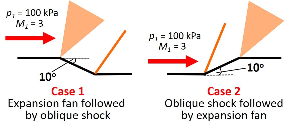
A uniform supersonic flow of a perfect gas with $\displaystyle \gamma$ = 1.4, Mach number 3.0 and an upstream static pressure of 100 kPa flows over a geometry as shown below. Determine the downstream static pressure for each case.

To analyze case 1, we divide the flow into three regions, as shown.

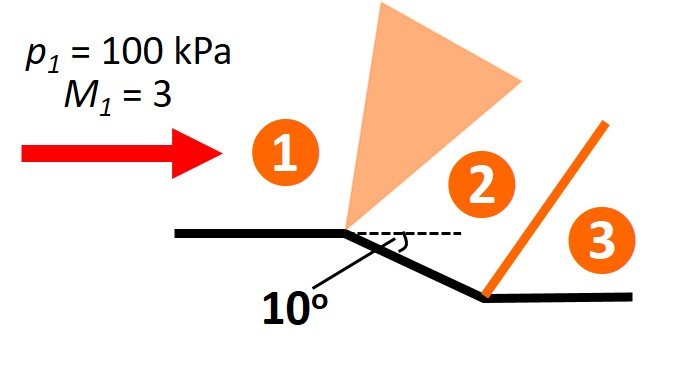
In region 1, from the Prandtl-Meyer table at $\displaystyle \gamma$ = 1.4 and M₁ = 3.0, we read v₁ = 49.7573^o. Using an isentropic flow table, we read a pressure ratio p₁/p₀₁ = 0.02722. Region 2 is reached by passing through an expansion fan in which the flow is turned back 10^o. Accordingly, we enter v₂ = v₁ + 10^o = 59.7573^o into the Prandtl-Meyer table to read M₂ $\displaystyle \approx$ 3.58 (the closest entry is for an angle of 59.7838^o). Then, we enter this Mach number into an isentropic flow table to read a pressure ratio p₂/p₀₂ = 0.0117. Because an expansion fan is isentropic, the stagnation pressure remains unchanged and p₀₂/p₀₁ = 1. Now, region 3 is reached by passing through an oblique shock in which the flow is turned back 10^o. Entering M₂ = 3.58 and $\displaystyle \delta$ = 10^o into an oblique shock table or chart, we read M₃ = 2.982 and p₃/p₂ = 2.315. We are now in position to compute downstream static pressure p₃,

$\displaystyle {{p}_{3}}=\frac{{{{p}_{3}}}}{{{{p}_{2}}}}\frac{{{{p}_{2}}}}{{{{p}_{{o2}}}}}\frac{{{{p}_{{o2}}}}}{{{{p}_{{o1}}}}}\frac{{{{p}_{{o1}}}}}{{{{p}_{1}}}}{{p}_{1}}$

$\displaystyle {{p}_{3}}=2.315\times 0.0117\times 1\times \frac{1}{{0.02722}}\times 100=99.51\,\text{kPa}\leftarrow$

We now turn to case 2, which we divide into three regions as before.

Region 2 is reached by passing through an oblique shock in which the flow is turned through 10^o. Referring to an oblique shock table or chart with M₁ = 3.0 and $\displaystyle \delta$ = 10^o, we read M₂ = 2.505 and p₂/p₁ = 2.054. Also, p₀₂/p₀₁ = 0.9631. After the oblique shock, the flow evolves isentropically through region 2 at a Mach number M₂. Entering M₂ = 2.505 into an isentropic flow table, we read p₂/p₀₂ = 0.0585 (the closest entry I found was for M₂ = 2.50). After reaching the top of the upwards-sloped section, the flow forms an expansion fan before spreading to region 3. Entering M₂ = 2.505 into the Prandtl-Meyer table, we read v₂ = 39.1236^o (again, the closest entry in the table is for M₂ = 2.50). As the flow is turned 10^o when expanding to region 3, we may write v₃ = v₂ + 10^o = 49.1236^o. Entering this angle into the Prandtl-Meyer table, we read a Mach number M₃ = 2.96 (the closest entry is for an angle of 48.9796^o). Referring to an isentropic table one last time, we enter M₃ = 2.96 to read p₃/p₀₃ = 0.0289. We can glean our results and compute downstream static pressure p_3,

$\displaystyle {{p}_{3}}=\frac{{{{p}_{3}}}}{{{{p}_{{o3}}}}}\frac{{{{p}_{{o3}}}}}{{{{p}_{{o2}}}}}\frac{{{{p}_{{o2}}}}}{{{{p}_{2}}}}\frac{{{{p}_{2}}}}{{{{p}_{1}}}}{{p}_{1}}$

$\displaystyle {{p}_{3}}=0.0289\times 1\times \frac{1}{{0.0585}}\times 2.054\times 100=101.47\,\text{kPa}\leftarrow$

In short, the arrangement in case 1 ultimately leads to a decrease in pressure of about 0.5% relatively to initial pressure, while case 2 culminates with an increase close to 1.5%.

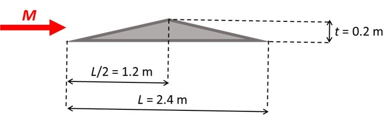
Example problem 3

A two-dimensional supersonic wing has the profile illustrated below. At zero angle of attack, determine the drag force on the wing per unit length of span at Mach 2. Repeat for lift force. Take the maximum thickness of the airfoil to be 0.2 m.

Let the regions involved in the calculations be numbered as follows. An oblique shock occurs as the flow transitions from 1 to 2; a Prandtl-Meyer expansion fan occurs as the flow transitions from 2 to 3; lastly, a second oblique shock occurs as the flow transitions from 3 to 4.

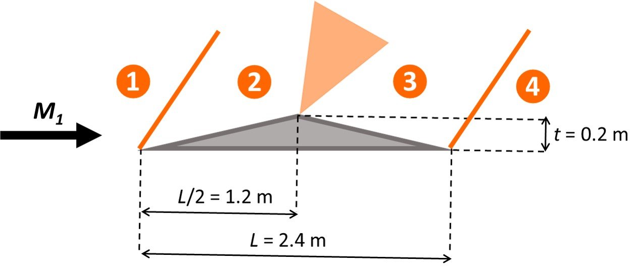
Flow reaches the airfoil at Mach number M₁ = 2.0 and deflection angle $\displaystyle \delta$ such that

$\displaystyle \delta ={{\tan }^{{-1}}}\left( {\frac{t}{{{L}/{2}\;}}} \right)={{\tan }^{{-1}}}\left( {\frac{{0.2}}{{{{2.4}}/{2}\;}}} \right)=9.462{}^\text{o}$

At this Mach number and deflection angle, refer to an oblique shock table or chart to read a wave angle $\displaystyle \beta$ = 38.78^o, a downstream Mach number M₂ = 1.659, and a pressure ratio p₂/p₁ = 1.664. Entering M₂ into an isentropic flow table, we get the static-to-stagnation pressure ratio p₂/p₀₂ = 0.2151 (the closest entry is for M₂ = 1.66). As the flow transitions from 2 to 3, an expansion fan is formed. Entering M₂ = 1.66 into the Prandtl-Meyer table, we read v₂ = 16.6328^o (again, the closest entry is for M₂ = 1.66). Now, as the flow moves from region 2 to 3 it turns 2 $\displaystyle \delta$ = 2 $\displaystyle \times$ 9.462^o = 18.924^o, so the Prandtl-Meyer function at 3 becomes

$\displaystyle {{v}_{3}}={{v}_{2}}+2\delta =16.6328{}^\text{o}+18.924{}^\text{o}=35.5568{}^\text{o}$

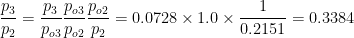
Entering this value into a Prandtl-Meyer table yields M₃ = 2.36 (the closest entry is for v = 35.7715^o). Taking this Mach number into an isentropic flow table one last time gives a static-to-stagnation pressure ratio p₃/p₀₃ = 0.0728. The flow goes on to form a second oblique shock at the trailing edge of the airfoil, but our results so far suffice to compute pressures p₁, p₂, and p₃, which are all we need to compute the lift and drag forces on the foil. Thus, we ignore calculations for the transition from 3 to 4. Gleaning results, we write

$\displaystyle \frac{{{{p}_{3}}}}{{{{p}_{2}}}}=\frac{{{{p}_{3}}}}{{{{p}_{{o3}}}}}\frac{{{{p}_{{o3}}}}}{{{{p}_{{o2}}}}}\frac{{{{p}_{{o2}}}}}{{{{p}_{2}}}}=0.0728\times 1.0\times \frac{1}{{0.2151}}=0.3384$

At region 1, flow pressure equals the free-stream pressure, that is,

$\displaystyle {{p}_{1}}={{p}_{\infty }}=20\,\text{kPa}$

At region 2, flow pressure is

$\displaystyle {{p}_{2}}=\left( {\frac{{{{p}_{2}}}}{{{{p}_{1}}}}} \right){{p}_{1}}=1.664\times 20=33.28\,\text{kPa}$

Lastly, at region 3

$\displaystyle {{p}_{3}}=\left( {\frac{{{{p}_{3}}}}{{{{p}_{2}}}}} \right){{p}_{2}}=0.3384\times 33.28=11.26\,\text{kPa}$

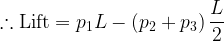
Now, the drag force acting on the foil consists of two contributions, one from each half of the upper camber; mathematically,

$\displaystyle \text{Drag}={{p}_{2}}\left( {\frac{t}{{\sin \delta }}} \right)\sin \delta -{{p}_{3}}\left( {\frac{t}{{\sin \delta }}} \right)\sin \delta$

$\displaystyle \therefore \text{Drag}=\left( {{{p}_{2}}-{{p}_{3}}} \right)t$

$\displaystyle \therefore \text{Drag}=\left( {33.28-11.26} \right)\times 0.2=4.40\,\text{kN/m}\leftarrow$

The lift force, in turn, includes not only the contributions from the two halves of the upper camber, but also one from the flat lower camber; in mathematical terms,

$\displaystyle \text{Lift}={{p}_{1}}L-{{p}_{2}}\left( {\frac{t}{{\sin \delta }}} \right)\cos \delta -{{p}_{3}}\left( {\frac{t}{{\sin \delta }}} \right)\cos \delta$

$\displaystyle \therefore \text{Lift}={{p}_{1}}L-\left( {{{p}_{2}}+{{p}_{3}}} \right)\frac{L}{2}$

$\displaystyle \therefore \text{Lift}=20\times 2.4-\left( {33.28+11.26} \right)\times \frac{{2.4}}{2}=-5.45\,\text{kN/m}\leftarrow$

The negative sign indicates that the lift is actually pointing downward.

Go further

Those looking for more solved problems on shock theory might want to check out our free quiz on normal and oblique shock waves, which you can find here.

References

• ANDERSON, J.D., JR. (2011). Fundamentals of Aerodynamics. 5th edition. New York: McGraw-Hill.

• BABU, V. (2021). Fundamentals of Gas Dynamics. 2nd edition. Berlin/Heidelberg: Springer.

• JOHN, J.E. and KEITH, T.G. (2006). Gas Dynamics. 3rd edition. Upper Saddle River: Pearson Prentice Hall.

Prandtl-Meyer Expansion Waves: Derivation and Problems

Subscribe to our Mailing List!

Featured Posts

A Primer on NAND Flash Memories

Solidification Time and Chvorinov’s Rule

Step-Growth Polymerization, the Carothers Equation, and the Flory-Schulz Distribution

More Articles

Cruise Flight Performance of Piston-Prop Aircraft

Plasticity: Tresca and von Mises Yield Criteria

Fields of Study

More

© 2024 Montogue Quiz

Subscribe to
our Mailing List!

Subscribe to our Mailing List!

Subscribe to receive our latest materials in your inbox.

Homework Help

© 2024 Montogue Quiz

Subscribe to our Mailing List!